PITcleanr Workshop
Ryan N. Kinzer
Mike Ackerman
Kevin See
Feb 1, 2024
Source:vignettes/PITcleanr_workshop.Rmd
PITcleanr_workshop.RmdIntroduction
PIT-tag data is often difficult to summarize into meaningful
information due to the large amount of tag observations. For instance,
PTAGIS serves as a data repository containing a single record for every
observation of a tag code; including the initial detection, or “mark”,
when the tag is implanted, and all subsequent detections on each antenna
the tag passes, or at recapture (e.g., at weirs), and recovery (e.g.,
carcass surveys) sites. The number of detections that exist for each
individual tag code can easily be in excess of 1,000s of observations.
Therefore, querying PTAGIS for all detections of a large number of tags
often leads to a wealth of data that is unwieldy to process.
PITcleanr aims to “compress” or minimize the data to a more
manageable size, without losing any of the information contained in the
full dataset, and to provide useful tools to help organize the data into
fish pathways and stream networks.
This document serves as a tutorial to the most common functions
contained in PITcleanr and provides some simple data
summaries that may help you get started using the package, and
performing your own PIT-tag data analyses. The workshop contains four
sections:
- querying data,
- compressing tag observations,
- developing fish pathways, and finally,
- an example case study.
Additional information on PITcleanr can be found on its GitHub page or website. Materials from this workshop can be found here.
Installation
PITcleanr can be installed from GitHub using the R
remotes package. Additional information on package
installation can be found on the PITcleanr website README.
# install PITcleanr, if necessary
install.packages("remotes")
remotes::install_github("KevinSee/PITcleanr",
                        build_vignettes = TRUE)
Load Packages
Once PITcleanr is successfully installed it can be
loaded into the R session using the library() function. In
this workshop, we will also use functions from the following packages;
tidyverse, sf, and kableExtra.
Use the install.packages() function for packages that are
not already installed.
Query Site Data
Interrogation Sites
PITcleanr can be used to query and download metadata for
PTAGIS interrogation sites using the function
queryInterrogationMeta(). The site_code
argument is used to specify sites; alternatively, set
site_code = NULL to retrieve metadata for all sites.
# interrogation site metadata
int_meta_KRS = queryInterrogationMeta(site_code = "KRS") # South Fork Salmon River, Krassel
int_meta = queryInterrogationMeta(site_code = NULL)
As a simple example, after downloading the interrogation metadata you
can quickly summarize the number of active instream remote detections
systems in PTAGIS by organization using tidyverse
functions.
# count active instream remote sites by organization
int_meta %>%
  filter(siteType == "Instream Remote Detection System",
         active) %>%
  count(operationsOrganizationCode) %>%
  ggplot(aes(x = operationsOrganizationCode, y = n)) +
    geom_col() +
    coord_flip()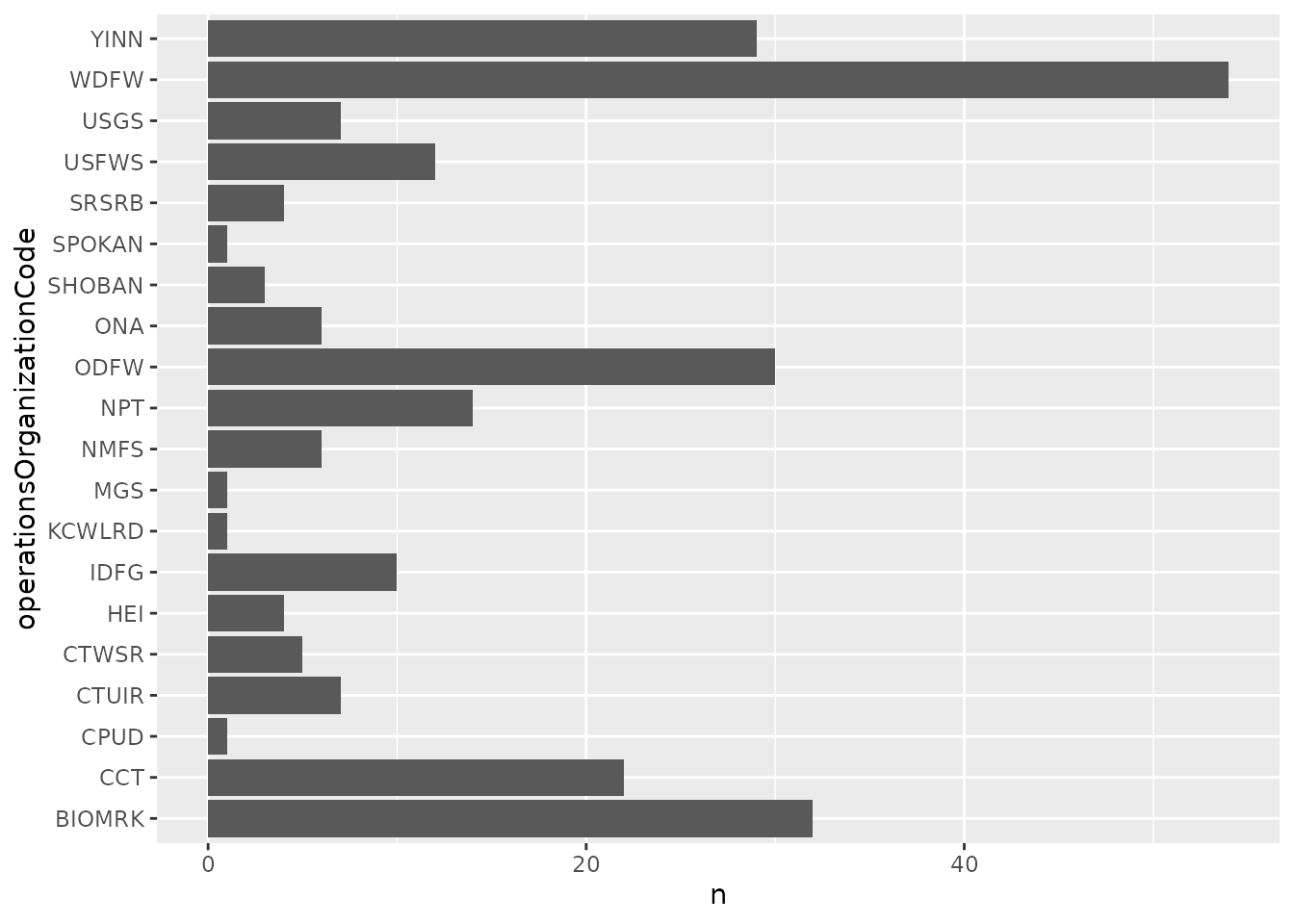
Or, we can use the int_meta object to map our
interrogation sites using the sf package. State polygons
are available from the maps package.
# plot location of interrogation sites
# install.packages('maps')

# get state boundaries
pnw <-
  st_as_sf(maps::map("state",
                     region = c('ID', 'WA', 'OR'),
                     plot = FALSE,
                     fill = TRUE))

# create spatial feature object of IPTDS
int_sf <-
  int_meta %>%
  filter(siteType == "Instream Remote Detection System",
         !is.na(longitude),
         !is.na(latitude)) %>%
  st_as_sf(coords = c('longitude', 'latitude'),
           crs = 4326) # WGS84

ggplot() +
  geom_sf(data = pnw) +
  geom_sf(data = int_sf, aes(color = active))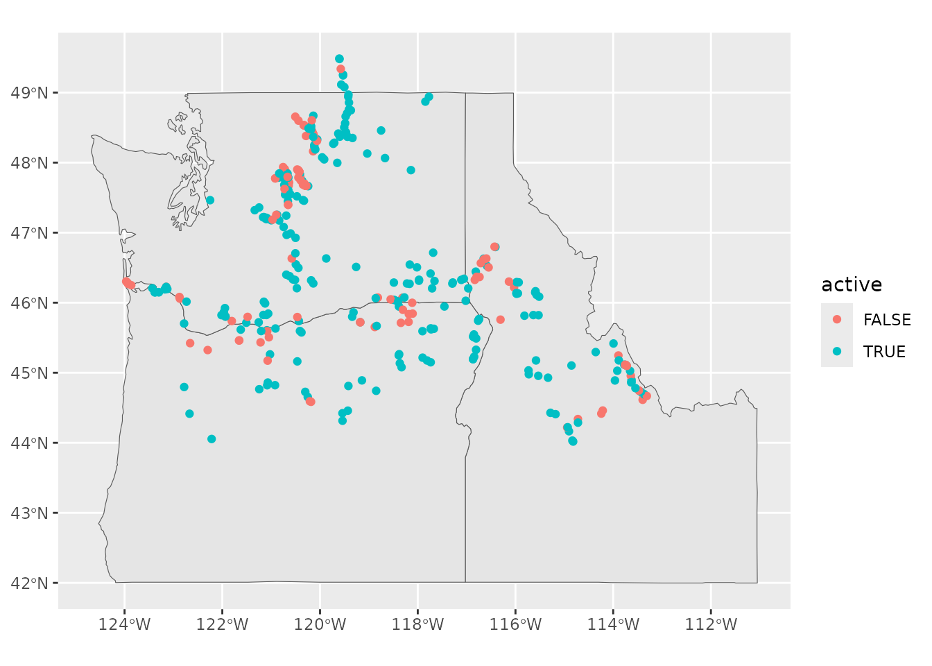
PITcleanr also includes the
queryInterrogationConfig() function to query and download
configuration metadata for PTAGIS interrogation sites. The configuration
metadata contains information about individual antennas, transceivers,
and their arrangement across time. Similar to above,
site_code can be set to NULL to get
configuration metadata for all PTAGIS interrogation sites or you can
designate the site of interest.
# configuration of an interrogation site
int_config <- queryInterrogationConfig(site_code = 'ZEN') # Secesh River, Zena Creek Ranch

int_config %>%
  kable() %>%
  kable_styling(full_width = TRUE,
bootstrap_options = 'striped')| siteCode | siteName | siteType | configurationSequence | startDate | endDate | isCurrent | antennaGroupName | antennaGroupSortValue | transceiverID | transceiverType | antennaID |
|---|---|---|---|---|---|---|---|---|---|---|---|
| ZEN | Secesh River at Zena Cr. Ranch | Instream | 110 | 2012-04-12 | NA | TRUE | UPPER IN-STREAM ARRAY | A | A0 | FS1001M | A1 |
| ZEN | Secesh River at Zena Cr. Ranch | Instream | 110 | 2012-04-12 | NA | TRUE | UPPER IN-STREAM ARRAY | A | A0 | FS1001M | A2 |
| ZEN | Secesh River at Zena Cr. Ranch | Instream | 110 | 2012-04-12 | NA | TRUE | UPPER IN-STREAM ARRAY | A | A0 | FS1001M | A3 |
| ZEN | Secesh River at Zena Cr. Ranch | Instream | 110 | 2012-04-12 | NA | TRUE | UPPER IN-STREAM ARRAY | A | A0 | FS1001M | A4 |
| ZEN | Secesh River at Zena Cr. Ranch | Instream | 110 | 2012-04-12 | NA | TRUE | LOWER IN-STREAM ARRAY | B | B0 | Unknown | B1 |
| ZEN | Secesh River at Zena Cr. Ranch | Instream | 110 | 2012-04-12 | NA | TRUE | LOWER IN-STREAM ARRAY | B | B0 | Unknown | B2 |
| ZEN | Secesh River at Zena Cr. Ranch | Instream | 110 | 2012-04-12 | NA | TRUE | LOWER IN-STREAM ARRAY | B | B0 | Unknown | B3 |
| ZEN | Secesh River at Zena Cr. Ranch | Instream | 110 | 2012-04-12 | NA | TRUE | LOWER IN-STREAM ARRAY | B | B0 | Unknown | B4 |
| ZEN | Secesh River at Zena Cr. Ranch | Instream | 110 | 2012-04-12 | NA | TRUE | LOWER IN-STREAM ARRAY | B | B0 | Unknown | B5 |
| ZEN | Secesh River at Zena Cr. Ranch | Instream | 110 | 2012-04-12 | NA | TRUE | LOWER IN-STREAM ARRAY | B | B0 | Unknown | B6 |
Mark/Recapture/Recovery Sites
A similar function exists to query and download metadata for PTAGIS
mark-recapture-recovery (MRR) sites; however, configuration data doesn’t
exist for MRR sites so there is no need for a
queryMRRConfig() function.
# all MRR sites
mrr_meta <- queryMRRMeta(site = NULL)

head(mrr_meta, 3) %>%
  kable() %>%
  kable_styling(full_width = TRUE,
bootstrap_options = "striped")| siteCode | name | rkm | type | huC8Code | latitude | longitude | coordinateType | legacyType | parentLocation | minKm | maxKm | markSiteOnly | pointLocation | shapeType | streamLocationId | spatialLineId | spatialPolyId | spatialFacId |
|---|---|---|---|---|---|---|---|---|---|---|---|---|---|---|---|---|---|---|
| 15MILC | Fifteen Mile Creek, near The Dalles, Oregon | 309 | River | 17070105 | 45.48169 | -121.0756 | Midpoint | R | 0 | 86 | FALSE | FALSE | line | 1211264456185 | 119 | NA | NA | |
| 1890SC | 1890s Side Channel Methow River | 843.067 | River | 17020008 | 48.37819 | -120.1331 | Midpoint | R | 0 | 3 | FALSE | FALSE | line | 1201196483692 | 586 | NA | NA | |
| 18MILC | Eighteenmile Creek, Lemhi River Basin | 522.303.416.092 | River | 17060204 | 44.52558 | -113.2369 | Midpoint | R | 0 | 43 | FALSE | FALSE | line | 1133545446822 | 145 | NA | NA |
All PTAGIS Sites
PITcleanr includes additional wrapper functions that can
query interrogation and MRR sites together. The
queryPtagisMeta() function downloads all INT and MRR sites
at once. The buildConfig() function goes a step further and
downloads all INT and MRR site metadata, plus INT site configuration
information, and then applies some formatting to combine all metadata
into a single data frame. Additionally, buildConfig()
creates a node field which can be used to assign and group
detections to a user-specified spatial scale.
# wrapper to download all site meta
# ptagis_meta <- queryPtagisMeta()

# wrapper to download site metadata and INT configuration data at once, and apply some formatting
config <- buildConfig(node_assign = "array",
                      array_suffix = "UD")

# number of unique sites in PTAGIS
n_distinct(config$site_code)
#> [1] 2000

# number of unique nodes in PTAGIS
n_distinct(config$node)
#> [1] 2283

# the number of detection locations/antennas in PTAGIS
nrow(config)
#> [1] 7906

head(config, 9) %>%
  select(-site_description) %>% # remove site_description column for formatting
  kable() %>%
  kable_styling(full_width = TRUE,
bootstrap_options = "striped")| site_code | config_id | antenna_id | node | start_date | end_date | site_type | site_name | antenna_group | site_type_name | rkm | rkm_total | latitude | longitude |
|---|---|---|---|---|---|---|---|---|---|---|---|---|---|
| 0HR | 100 | 01 | 0HR | 2022-07-26 | NA | INT | Henrys Instream Array | Main Array | Instream Remote Detection System | 522.303.416.047 | 1288 | 44.89690 | -113.6247 |
| 0HR | 100 | 02 | 0HR | 2022-07-26 | NA | INT | Henrys Instream Array | Main Array | Instream Remote Detection System | 522.303.416.047 | 1288 | 44.89690 | -113.6247 |
| 0HR | 100 | 03 | 0HR | 2022-07-26 | NA | INT | Henrys Instream Array | Main Array | Instream Remote Detection System | 522.303.416.047 | 1288 | 44.89690 | -113.6247 |
| 158 | 100 | D1 | 158_U | 2011-11-29 | NA | INT | Fifteenmile Ck at Eightmile Ck | Upstream Eightmile Ck | Instream Remote Detection System | 309.004 | 313 | 45.60643 | -121.0863 |
| 158 | 100 | D2 | 158_U | 2011-11-29 | NA | INT | Fifteenmile Ck at Eightmile Ck | Middle Eightmile Ck | Instream Remote Detection System | 309.004 | 313 | 45.60643 | -121.0863 |
| 158 | 100 | D3 | 158_D | 2011-11-29 | NA | INT | Fifteenmile Ck at Eightmile Ck | Downstream Eightmile Ck | Instream Remote Detection System | 309.004 | 313 | 45.60643 | -121.0863 |
| 158 | 100 | D4 | 158_U | 2011-11-29 | NA | INT | Fifteenmile Ck at Eightmile Ck | Upstream Fifteenmile Ck | Instream Remote Detection System | 309.004 | 313 | 45.60643 | -121.0863 |
| 158 | 100 | D5 | 158_U | 2011-11-29 | NA | INT | Fifteenmile Ck at Eightmile Ck | Middle Fifteenmile Ck | Instream Remote Detection System | 309.004 | 313 | 45.60643 | -121.0863 |
| 158 | 100 | D6 | 158_D | 2011-11-29 | NA | INT | Fifteenmile Ck at Eightmile Ck | Downstream Fifteenmile Ck | Instream Remote Detection System | 309.004 | 313 | 45.60643 | -121.0863 |
The buildConfig() column includes the arguments
node_assign and array_suffix. The node_assign
argument includes the options c("array", "site", "antenna")
which allows the user to assign PIT tag arrays, entire sites, or
individual antennas, respectively, as nodes, which can then
be used as a grouping variable for subsequent data prep and analysis. In
the case node_assign = "array", the
array_suffix can be used to assign suffixes to each PIT-tag
array. By default, observations are assigned to individual arrays, and
upstream and downstream arrays are assigned the suffixes “_U” and “_D”,
respectively. In the case of 3-span arrays, observations at the middle
array are assigned to the upstream array. Play with the different
settings and review the output to learn the differences.
tmp_config <- buildConfig(node_assign = "site") # c("array", "site", "antenna)

# The option to use "UMD" is still in development.
tmp_config <- buildConfig(node_assign = "array",
                          array_suffix = "UMD") # c("UD", "UMD", "AOBO")
Test Tags
To help assess a site’s operational condition PITcleanr
includes the function queryTimerTagSite(). The function
queries the timer test tag history from PTAGIS for a single
interrogation site during a calendar year. The test tag information is
useful to quickly examine the site for operation conditions and to help
understand potential assumption violations with future analyses.
# check for timer tag to evaluate site operation
test_tag <-
  queryTimerTagSite(site_code = "ZEN",
                    year = 2023,
                    api_key = my_api_key) # requires an API key

test_tag %>%
  ggplot(aes(x = time_stamp, y = 1)) +
  geom_point() +
  theme(axis.text.x = element_text(angle = -45, vjust = 0.5),
        axis.text.y = element_blank(),
        axis.ticks.y = element_blank(),
        axis.title.x = element_blank(),
        axis.title.y = element_blank()) +
  facet_grid(antenna_id ~ transceiver_id)
Compressing Tag Observations
PTAGIS Complete Tag Histories
In a typical PIT tag analysis workflow a user starts with a list of tags containing all the codes of interest, and then searches a data repository for all the observations of the listed tags.
Tag List
A tag list is typically a .txt file with one row per tag code. For
convenience, we’ve included one such file with PITcleanr,
which contains tag IDs for Chinook salmon adults implanted with tags at
Tumwater Dam in 2018. The following can be used to find the path to this
example file. Alternatively, the user can provide the file path to their
own tag list.
# generate file path to example tag list in PITcleanr
tag_list = system.file("extdata",
                       "TUM_chnk_tags_2018.txt",
                       package = "PITcleanr",
                       mustWork = TRUE)

read_delim(tag_list, delim='\t') %>%
  head(5) %>%
  kable(col.names = NULL) %>%
  kable_styling(full_width = TRUE,
bootstrap_options = "striped")| 3DD.00777C5E34 |
| 3DD.00777C7728 |
| 3DD.00777C8493 |
| 3DD.00777C9185 |
| 3DD.00777C91C3 |
# or simple example to your own file on desktop
#tag_list = "C:/Users/username/Desktop/my_tag_list.txt"
Read PTAGIS CTH
Once the user has created their own tag list, or located the above example, load the list into PTAGIS to query the complete tag history for each of the listed tags. Detailed instructions for querying complete tag histories in PTAGIS for use in PITcleanr can be found here. The following fields or attributes are required in the PTAGIS complete tag history query:
- Tag
- Event Site Code
- Event Date Time
- Antenna
- Antenna Group Configuration
Other available PTAGIS fields of interest may also be included. We highly recommended the following fields to help with future summaries:
- Mark Species
- Mark Rear Type
- Event Type
- Event Site Type
- Event Release Site Code
- Event Release Date Time
For convenience, we’ve included an example complete tag history in
PITcleanr from the above tag list, or you can provide the
file path to your own complete tag history.
# file path to the example CTH in PITcleanr
ptagis_file <- system.file("extdata",
                          "TUM_chnk_cth_2018.csv",
                          package = "PITcleanr",
                          mustWork = TRUE)
The PITcleanr function readCTH() is used to
read in your complete tag history. Once the data is read by
readCTH() it then re-formats the column names to be
consistent with subsequent PITcleanr functions. In the following example
we are only interested in tag observations after the start of the adult
run year; so we use the filter() function to remove the
excess observations.
raw_ptagis = readCTH(ptagis_file,
                     file_type = "PTAGIS") %>%
  # filter for only detections after start of run year
  filter(event_date_time_value >= lubridate::ymd(20180301))

# number of detections
nrow(raw_ptagis)
#> [1] 13294

# number of unique tags
dplyr::n_distinct(raw_ptagis$tag_code)
#> [1] 1406
We can compare the downloaded complete tag history file with the
output of the readCTH function by looking at the first
couple rows of data.
head(raw_ptagis, 4) %>%
  kable() %>%
  kable_styling(full_width = TRUE,
bootstrap_options = "striped")| tag_code | event_site_code_value | event_date_time_value | antenna_id | antenna_group_configuration_value | mark_species_name | mark_rear_type_name | event_type_name | event_site_type_description | event_release_site_code_code | event_release_date_time_value | cth_count |
|---|---|---|---|---|---|---|---|---|---|---|---|
| 384.3B239AC47B | NAL | 2018-07-01 00:06:16 | 63 | 100 | Chinook | Wild Fish or Natural Production | Observation | Instream Remote Detection System | NA | NA | 1 |
| 384.3B239AC47B | UWE | 2018-06-23 22:03:13 | B2 | 110 | Chinook | Wild Fish or Natural Production | Observation | Instream Remote Detection System | NA | NA | 1 |
| 384.3B239AC47B | BO3 | 2018-05-18 09:36:59 | 18 | 110 | Chinook | Wild Fish or Natural Production | Observation | Adult Fishway | NA | NA | 1 |
| 384.3B239AC47B | BO3 | 2018-05-18 09:37:11 | 16 | 110 | Chinook | Wild Fish or Natural Production | Observation | Adult Fishway | NA | NA | 1 |
head(read_csv(ptagis_file), 4) %>%
  kable() %>%
  kable_styling(full_width = TRUE,
bootstrap_options = "striped")| Tag Code | Mark Species Name | Mark Rear Type Name | Event Type Name | Event Site Type Description | Event Site Code Value | Event Date Time Value | Antenna ID | Antenna Group Configuration Value | Event Release Site Code Code | Event Release Date Time Value | CTH Count |
|---|---|---|---|---|---|---|---|---|---|---|---|
| 384.3B239AC47B | Chinook | Wild Fish or Natural Production | Mark | River | NASONC | 3/1/2016 10:34:00 AM | NA | 0 | NASONC | 3/4/2016 5:00:00 PM | 1 |
| 384.3B239AC47B | Chinook | Wild Fish or Natural Production | Observation | Instream Remote Detection System | NAL | 7/1/2018 12:06:16 AM | 63 | 100 | NA | NA | 1 |
| 384.3B239AC47B | Chinook | Wild Fish or Natural Production | Observation | Instream Remote Detection System | UWE | 6/23/2018 10:03:13 PM | B2 | 110 | NA | NA | 1 |
| 384.3B239AC47B | Chinook | Wild Fish or Natural Production | Observation | Adult Fishway | BO3 | 5/18/2018 9:36:59 AM | 18 | 110 | NA | NA | 1 |
Note that readCTH() includes the argument
file_type which can be used to import data from Biomark’s
BioLogic (“Biologic_csv”) database or data downloaded directly from a
PIT-tag reader, in either a .log or .xlsx format (“raw”). These formats
may be useful for smaller studies or studies outside the Columbia River
Basin whose data may not be uploaded to PTAGIS.
Quality Control
The qcTagHistory() function can be used to perform basic
quality control on PTAGIS detections. Note it can be run on either the
file path to the complete tag histories or the data frame returned by
readCTH(). qcTagHistory() provides information
on disowned and orphan tags and information on the various release
groups included in the detections. For more information, see the PTAGIS FAQ website.
# using the complete tag history file path
qc_detections = qcTagHistory(ptagis_file)

# or the complete tag history tibble from readCTH()
qc_detections = qcTagHistory(raw_ptagis)

# view release batch information
qc_detections$rel_time_batches %>%
  kable() %>%
  kable_styling(full_width = TRUE,
bootstrap_options = "striped")| mark_species_name | year | event_site_type_description | event_type_name | event_site_code_value | n_tags | n_events | n_release | rel_greq_event | rel_ls_event | event_rel_ratio |
|---|---|---|---|---|---|---|---|---|---|---|
| Chinook | 2018 | Dam | Mark | TUM | 1350 | 1350 | 1339 | 1350 | 0 | 1.008215 |
| Chinook | 2018 | Dam | Recapture | TUM | 136 | 143 | 142 | 143 | 0 | 1.007042 |
| Chinook | 2018 | Intra-Dam Release Site | Mark | BONAFF | 18 | 12 | 12 | 18 | 0 | 1.000000 |
| Chinook | 2018 | Intra-Dam Release Site | Mark | WELLD2 | 2 | 2 | 2 | 2 | 0 | 1.000000 |
| Chinook | 2018 | Trap or Weir | Recapture | CHIW | 66 | 5 | 5 | 66 | 0 | 1.000000 |
| Chinook | 2018 | Trap or Weir | Recapture | CHIWAT | 11 | 8 | 8 | 12 | 0 | 1.000000 |
Single Tag Codes and Marking Files
Often you may be interested in observations for a single tag code. To
help with this, PITcleanr contains the
queryCapHist() function to query observations for a single
tag from DART’s mirrored data repository of PTAGIS. This function can be
helpful if you are interested in a small number of tag codes and want to
programmatically develop summaries. The function requires a tag code
input and will return observation data post marking.
# query PTAGIS complete tag history for a single tag code; some examples
tagID <- "3D6.1D594D4AFA" # IR3, GOJ, BO1 -> IR5
tagID <- "3DD.003D494091" # GRA, IR1 -> IML

tag_cth = queryCapHist(ptagis_tag_code = tagID)

# example to summarise CTH
tag_cth %>%
  group_by(event_type_name,
           event_site_code_value) %>%
  summarise(n_dets = n(),
            min_det = min(event_date_time_value),
            max_det = max(event_date_time_value)) %>%
  mutate(duration = difftime(max_det, min_det, units = "hours")) %>%
  kable() %>%
  kable_styling(full_width = TRUE,
bootstrap_options = 'striped') | event_type_name | event_site_code_value | n_dets | min_det | max_det | duration |
|---|---|---|---|---|---|
| Observation | GRA | 11 | 2023-06-08 14:30:48 | 2023-06-08 14:35:48 | 0.0833333 hours |
| Observation | IML | 3 | 2023-07-02 15:42:18 | 2023-07-03 08:16:29 | 16.5697222 hours |
| Observation | IR1 | 1 | 2023-06-13 15:52:29 | 2023-06-13 15:52:29 | 0.0000000 hours |
| Observation | IR2 | 1 | 2023-06-14 16:00:55 | 2023-06-14 16:00:55 | 0.0000000 hours |
| Observation | IR3 | 4 | 2023-06-24 11:24:12 | 2023-06-24 11:27:44 | 0.0588889 hours |
| Observation | IR4 | 8 | 2023-07-01 19:50:12 | 2023-07-01 20:49:50 | 0.9938889 hours |
| Recapture | IMNAHW | 1 | 2023-07-03 10:00:00 | 2023-07-03 10:00:00 | 0.0000000 hours |
DART no longer provides mark event information with a tag code’s
observation data. If the marking information is necessary you can change
the argument include_mark to TRUE to also
query the PTAGIS marking record. Note: including the mark record
requires a PTAGIS “API Key” which can be requested from the PTAGIS
API website.
cth_node <- queryCapHist(ptagis_tag_code = tagID,
                         include_mark = TRUE,
                         api_key = my_api_key)
Additionally, the queryMRRDataFile() function can be
used to query a raw MRR file from PTAGIS. NOTE: only the latest
corrected version of the MRR file is returned.
# MRR tag file summaries
#mrr_file <- "NBD15065.TUM"
mrr_file <- "JSW-2022-175-001.xml"

mrr_data <- queryMRRDataFile(mrr_file)

# summary of injuries
mrr_data %>%
  group_by(species_run_rear_type,
           text_comments) %>%
  filter(!is.na(text_comments)) %>% # remove NA comments
  count() %>%
  ggplot(aes(x = text_comments,
             y = n,
             fill = species_run_rear_type)) +
  geom_col() +
  coord_flip() +
  labs(title = paste0(unique(mrr_data$release_site), ' : ', mrr_file))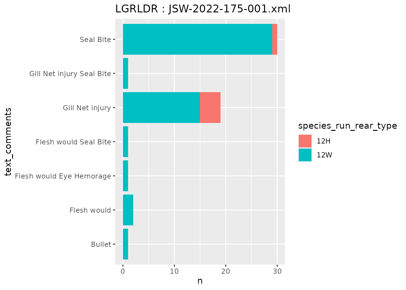
If more than one mark file is desired the user could iterate over
queryMRRDataFile() using purrr::map_df() to
query multiple files and combine them into a single data frame or
list.
julian = str_pad(1:10, 3, pad = 0) # julian 001 - 010
yr = 2024                          # tagging year

# Imnaha smolt trap, first 10 days of 2024
mrr_files = paste0("IMN-", yr, "-", julian, "-NT1.xml")

# iterate over files
mrr_data <- map_df(mrr_files,
             .f = queryMRRDataFile)

# view mrr data
head(mrr_data, 5)
#> # A tibble: 5 × 24
#>   capture_method event_date          event_site event_type life_stage
#>   <chr>          <dttm>              <chr>      <chr>      <chr>
#> 1 SCREWT         2024-01-01 12:00:00 IMNTRP     Tally      Juvenile
#> 2 SCREWT         2024-01-02 12:00:00 IMNTRP     Tally      Juvenile
#> 3 SCREWT         2024-01-03 08:59:12 IMNTRP     Mark       Juvenile
#> 4 SCREWT         2024-01-04 08:01:40 IMNTRP     Tally      Juvenile
#> 5 SCREWT         2024-01-04 08:04:06 IMNTRP     Mark       Juvenile
#> # ℹ 19 more variables: mark_method <chr>, migration_year <chr>,
#> #   organization <chr>, pit_tag <chr>, release_date <dttm>, release_site <chr>,
#> #   sequence_number <dbl>, species_run_rear_type <chr>, tagger <chr>,
#> #   n_fish <chr>, brood_year <chr>, length <dbl>, location_source <chr>,
#> #   location_latitude <chr>, location_longitude <chr>, mark_temperature <chr>,
#> #   release_temperature <chr>, weight <chr>, text_comments <chr>

# summarise new marks by day
mrr_data %>%
  filter(event_type == 'Mark') %>%
  mutate(release_date = date(release_date)) %>%
  group_by(release_date,
           species_run_rear_type) %>%
  count() %>%
  kable() %>%
  kable_styling(full_width = TRUE,
bootstrap_options = "striped")| release_date | species_run_rear_type | n |
|---|---|---|
| 2024-01-03 | 12W | 1 |
| 2024-01-04 | 12W | 2 |
| 2024-01-05 | 12W | 2 |
| 2024-01-08 | 12W | 5 |
| 2024-01-10 | 12W | 2 |
The mark data from queryMRRDataFile() and the
observations data from queryCapHist() could be combined to
form a complete tag history. However, this process is not recommended
for large number of tag codes.
Compress Detections
After downloading the complete tag history data from PTAGIS and
reading the file into the R environment with readCTH() we
are now ready to start summarizing the information. The first step is to
compress() the tag histories into a more manageable format
based on the “array” configuration from above using the function
buildConfg() and the arguments
node_assign == "array" and
array_suffix == "UD".
The compress() function assigns detections on individual
antennas to “nodes” (if no configuration file is provided, nodes are
considered site codes), summarizes the first and last detection time on
each node, as well as the number of detections that occurred during that
“slot”. More information on the compress() function can be
found here
or using ?PITcleanr::compress.
# compress observations
comp_obs <-
  compress(cth_file = raw_ptagis,
           configuration = config)

# view compressed observations
head(comp_obs)
#> # A tibble: 6 × 9
#>   tag_code       node   slot event_type_name n_dets min_det
#>   <chr>          <chr> <int> <chr>            <int> <dttm>
#> 1 384.3B239AC47B BO3       1 Observation         18 2018-05-18 09:36:59
#> 2 384.3B239AC47B BO4       2 Observation          7 2018-05-18 13:03:11
#> 3 384.3B239AC47B TD1       3 Observation          4 2018-05-20 17:20:39
#> 4 384.3B239AC47B JO1       4 Observation          2 2018-05-21 17:49:21
#> 5 384.3B239AC47B MC2       5 Observation         12 2018-05-24 09:04:38
#> 6 384.3B239AC47B PRA       6 Observation          4 2018-05-28 13:58:51
#> # ℹ 3 more variables: max_det <dttm>, duration <drtn>, travel_time <drtn>

# compare number of detections
nrow(raw_ptagis)
#> [1] 13294
nrow(comp_obs)
#> [1] 6755
The result of compress() can summarized in a variety of
ways, including the number of unique tags at each node.
n_distinct(comp_obs$tag_code)
#> [1] 1406

# number of unique tags per node
comp_obs %>%
  group_by(node) %>%
  summarise(n = n_distinct(tag_code)) %>%
  ggplot(aes(x = fct_reorder(node,n), y = n)) +
  geom_col() +
  coord_flip()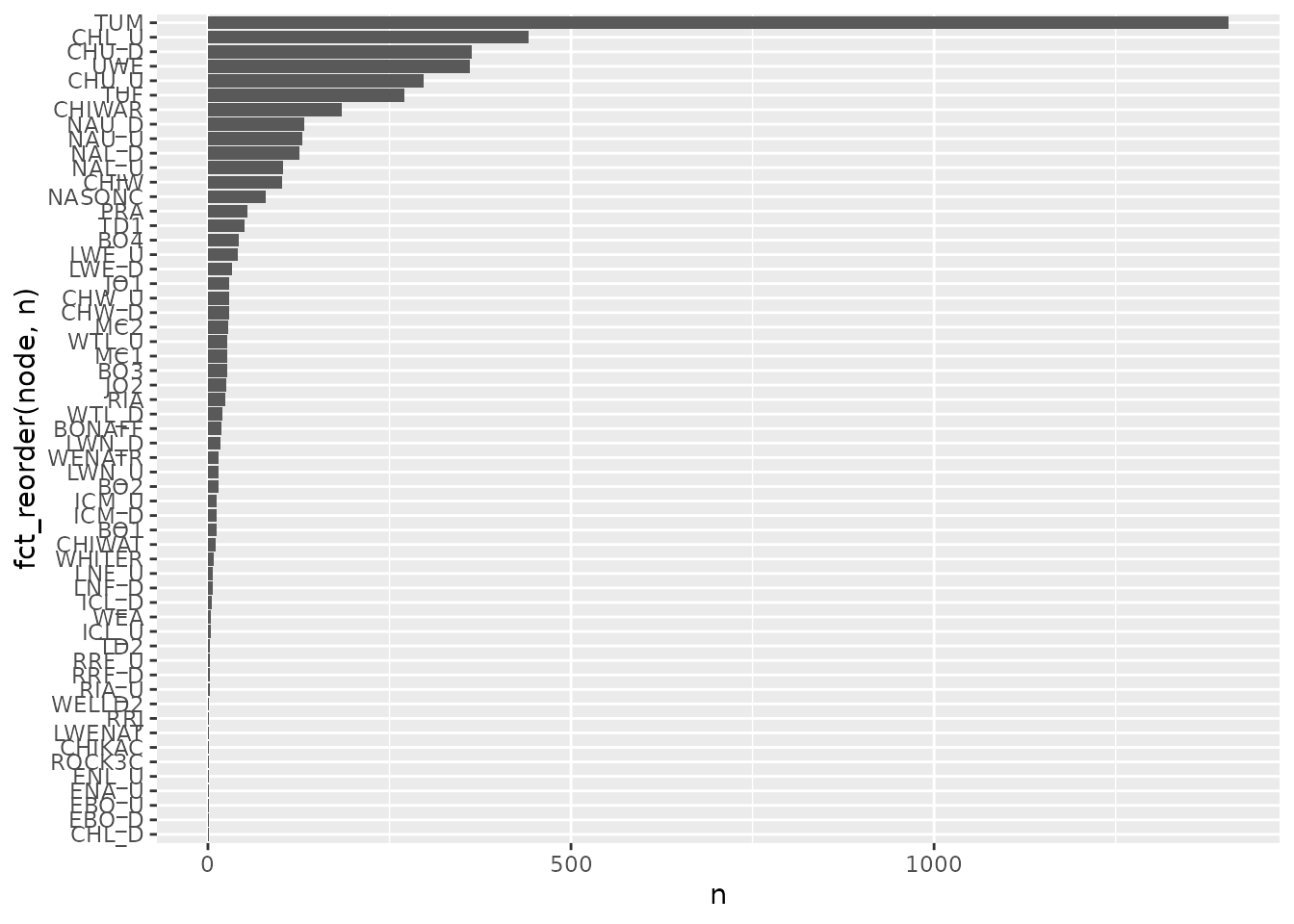
Compressing individual antenna detections to a more useful spatial scale and a more manageable size and format is a useful initial step. Further, summaries of compressed detections can answer some questions. However, more meaningful inference from PIT-tag data often requires understanding the relationship of your sites or nodes to one another, to better understand fish movements.
Fish Pathways
Parent-Child Tables
A next typical step in a PIT-tag analysis within a stream or river
network is to order the nodes, or observation sites, along the network
using their location. Ordering observations is completed using a
“parent-child” table. To create a parent-child table, we first need to
extract the sites of interest and place them on the stream using the
lat/long data stored in PTAGIS. The PITcleanr function
extractSites() can be used to extract detection sites from
your complete tag history file. Setting as_sf == T will
return your data frame as a simple
features object using the sf package.
# extract sites from complete tag histories
sites_sf <-
  extractSites(cth_file = raw_ptagis,
               as_sf = T,
               min_date = '20180301',
               configuration = config)
After reviewing the data you may find that some sites should be
removed or renamed for your particular analysis. This step can easily be
accomplished with tidyverse commands. For our example, we
are only interested in interrogation sites upstream of Tumwater Dam, and
we want to combine both Tumwater detection sites; TUM and TUF.
sites_sf <-
  sites_sf %>%
  # all sites in Wenatchee have an rkm greater than or equal to 754
  filter(str_detect(rkm, '^754'),
         type != "MRR",            # ignore MRR sites
         site_code != 'LWE') %>%   # ignore a site downstream of Tumwater
  mutate(across(site_code,
                ~ recode(.,
                         "TUF" = "TUM"))) # combine TUM and TUF
The next step is to download the stream spatial layer from the USGS
and the National
Hydrography Dataset. The stream layer is downloaded using the
queryFlowlines() function and is structured as a list that
needs to be converted into an sf object.
# download subset of NHDPlus flowlines
nhd_list <-
queryFlowlines(sites_sf = sites_sf,
root_site_code = "TUM",
min_strm_order = 2,
combine_up_down = TRUE)
# extract flowlines flowlines nhd_list
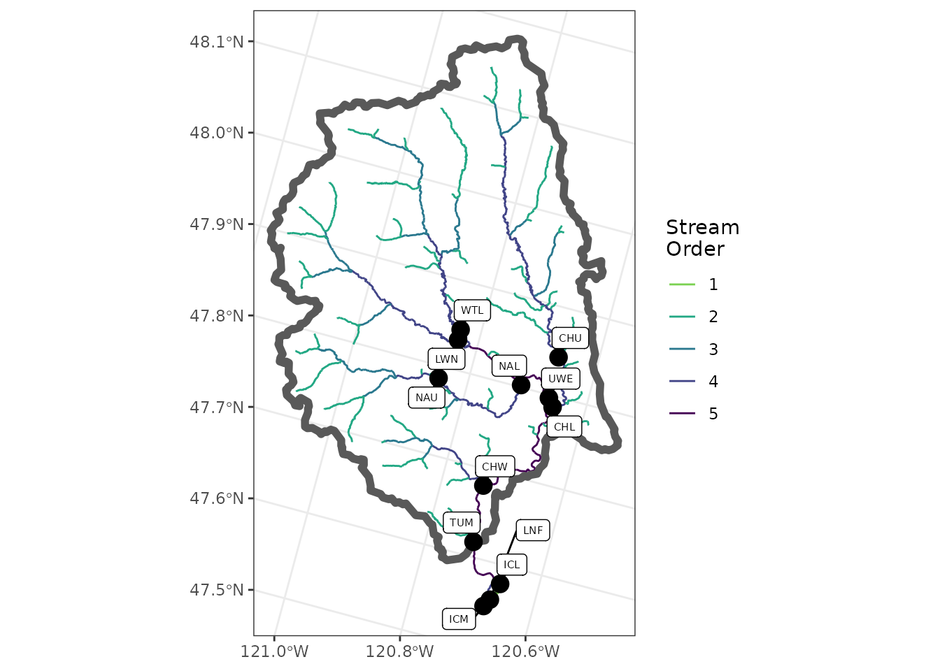
flowlines <- nhd_list$flowlinesThe sites_sf and flowlines objects can now
be used to create a simple map of your site locations which can be used
to understand how nodes or sites relate to each other across the stream
network.
# load ggplot
library(ggplot2)

tum_map <- ggplot() +
  geom_sf(data = flowlines,
          aes(color = as.factor(streamorde),
              size = streamorde)) +
  scale_color_viridis_d(direction = -1,
                        option = "D",
                        name = "Stream\nOrder",
                        end = 0.8) +
  scale_size_continuous(range = c(0.2, 1.2),
                        guide = 'none') +
  geom_sf(data = nhd_list$basin,
          fill = NA,
          lwd = 2) +
  theme_bw() +
  theme(axis.title = element_blank())

tum_map +
  geom_sf(data = sites_sf,
          size = 4,
          color = "black") +
  ggrepel::geom_label_repel(
    data = sites_sf,
    aes(label = site_code,
        geometry = geometry),
    size = 2,
    stat = "sf_coordinates",
    min.segment.length = 0,
    max.overlaps = 50
  )
These same objects can also be used to construct the parent-child
table using buildParentChild(). The parent-child table is
necessary to understand whether fish movements are upstream or
downstream, and is used frequently in further processing of your PIT-tag
observations.
# build parent-child table
parent_child = buildParentChild(sites_sf,
                                flowlines)
After building the parent-child table from the complete tag history
data and its extracted sites, we recommend plotting the nodes to
double-check all the locations of interest are included. The
relationship of nodes to each other can be easily plotted with the
plotNodes() function.
# plot parent-child table
plotNodes(parent_child)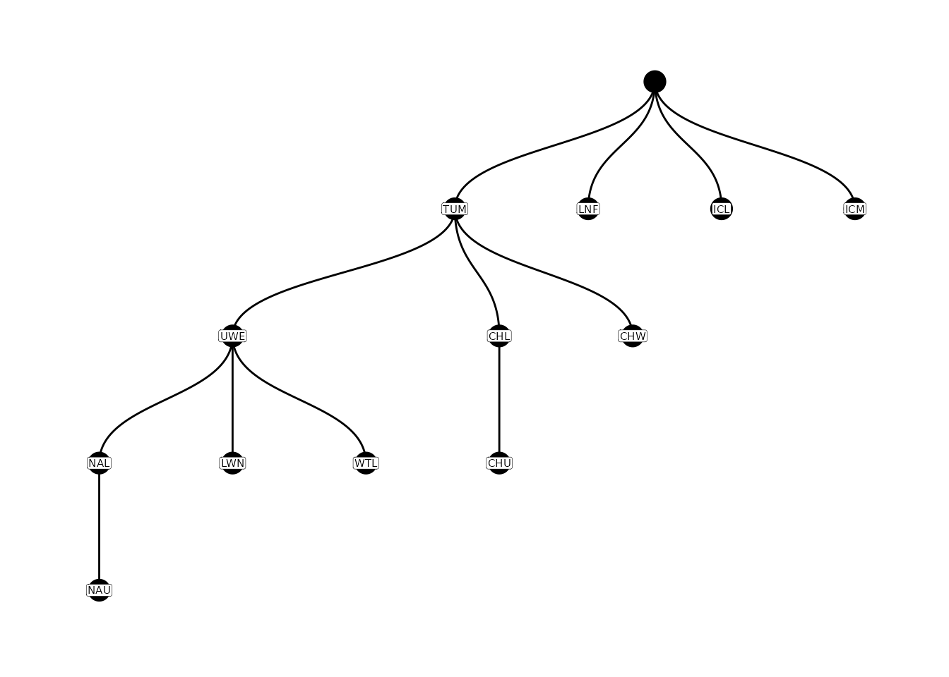
Sometimes errors occur in the parent-child table (e.g., due to errors
in lat/lon data, points being “snapped” poorly to flowlines). In this
case, the parent-child table can be edited using the
editParentChild() function. Additional details regarding
these functions can be found here.
# edit parent-child table
parent_child <-
  editParentChild(parent_child,
                  fix_list = list(c(NA, "LNF", "ICL"),
                                  c(NA, "ICL", "TUM"),
                                  c(NA, "ICM", "ICL")),
                  switch_parent_child = list(c("ICL", 'TUM'))) %>%
  filter(!is.na(parent))
# plot new parent-child table
plotNodes(parent_child)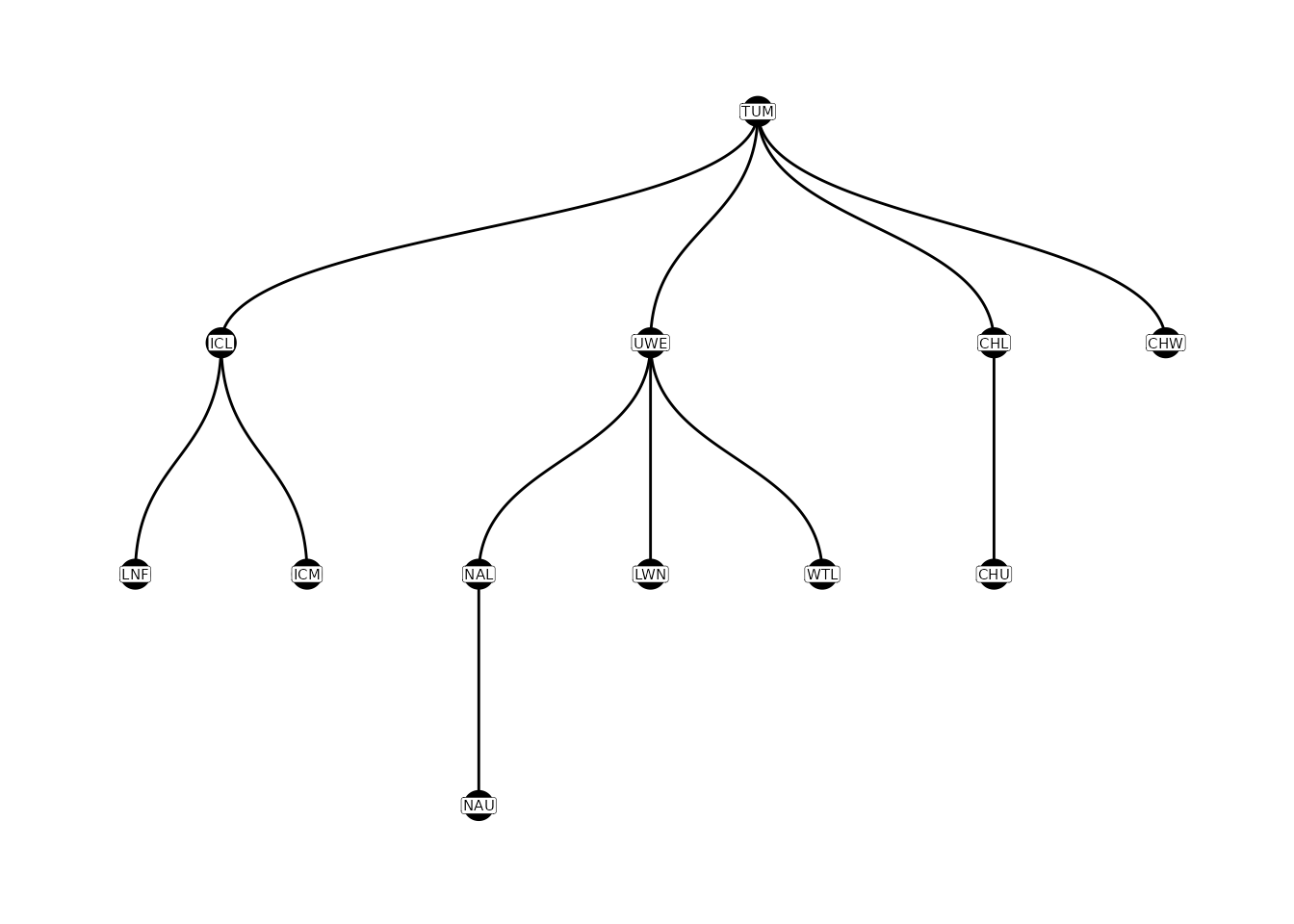
Add Nodes (Arrays)
If the configuration file contains multiple nodes for some sites
(e.g., a node for each array at a site), then the parent-child table can
be expanded to accommodate these nodes using the
addParentChildNodes() function.
# add nodes for arrays
parent_child_nodes <-
  addParentChildNodes(parent_child = parent_child,
                      configuration = config)

# plot parent-child w/ nodes
plotNodes(parent_child_nodes)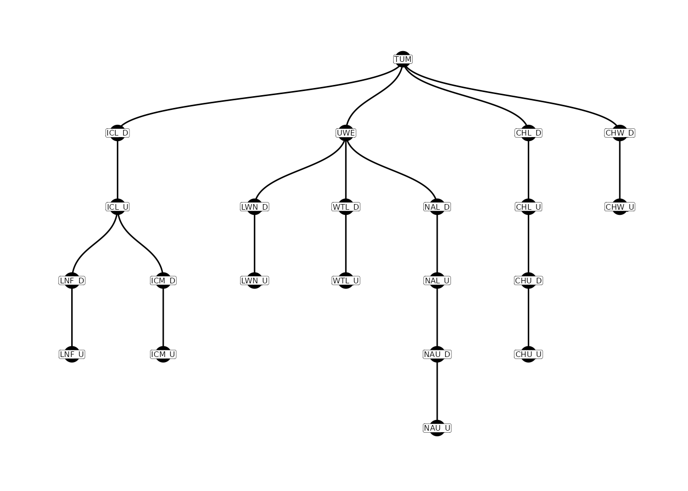
Movement Paths
PITcleanr provides two functions to determine the
detection locations a tag would need to pass between a starting point
(e.g., a tagging or release location) and an ending point (e.g., each
subsequent upstream or downstream detection point), based on the
parent-child table. We refer to these detection locations as a movement
path. They are equivalent to following one of the paths in the figures
above. The buildPaths() function creates the path, and
buildNodeOrder() goes one additional step and assigns the
node’s order in the pathway. Each of these functions includes the
argument direction which can be used to provide paths and
node orders based on upstream (e.g., adults; the default) or downstream
(e.g., juvenile) movements. For downstream movement, each node may
appear in the resulting tibble multiple times, as there may be multiple
ways to reach that node, from different starting points.
# build paths and add node order
node_order <-
  buildNodeOrder(parent_child = parent_child_nodes,
                 direction = "u")

# view node paths and orders
node_order %>%
  arrange(node) %>%
  kable() %>%
  kable_styling(full_width = TRUE,
bootstrap_options = "striped")| node | node_order | path |
|---|---|---|
| CHL_D | 2 | TUM CHL_D |
| CHL_U | 3 | TUM CHL_D CHL_U |
| CHU_D | 4 | TUM CHL_D CHL_U CHU_D |
| CHU_U | 5 | TUM CHL_D CHL_U CHU_D CHU_U |
| CHW_D | 2 | TUM CHW_D |
| CHW_U | 3 | TUM CHW_D CHW_U |
| ICL_D | 2 | TUM ICL_D |
| ICL_U | 3 | TUM ICL_D ICL_U |
| ICM_D | 4 | TUM ICL_D ICL_U ICM_D |
| ICM_U | 5 | TUM ICL_D ICL_U ICM_D ICM_U |
| LNF_D | 4 | TUM ICL_D ICL_U LNF_D |
| LNF_U | 5 | TUM ICL_D ICL_U LNF_D LNF_U |
| LWN_D | 3 | TUM UWE LWN_D |
| LWN_U | 4 | TUM UWE LWN_D LWN_U |
| NAL_D | 3 | TUM UWE NAL_D |
| NAL_U | 4 | TUM UWE NAL_D NAL_U |
| NAU_D | 5 | TUM UWE NAL_D NAL_U NAU_D |
| NAU_U | 6 | TUM UWE NAL_D NAL_U NAU_D NAU_U |
| TUM | 1 | TUM |
| UWE | 2 | TUM UWE |
| WTL_D | 3 | TUM UWE WTL_D |
| WTL_U | 4 | TUM UWE WTL_D WTL_U |
Travel Direction
With the parent-child relationships established,
PITcleanr can assign a movement direction between each node
where a given tag was detected using the function
addDirection().
# add direction based on parent-child table
comp_dir <-
  addDirection(compress_obs = comp_obs,
               parent_child = parent_child_nodes,
               direction = "u")

head(comp_dir, 6) %>%
  kable() %>%
  kable_styling(full_width = TRUE,
bootstrap_options = "striped")| tag_code | node | slot | event_type_name | n_dets | min_det | max_det | duration | travel_time | node_order | path | direction |
|---|---|---|---|---|---|---|---|---|---|---|---|
| 384.3B239AC47B | TUM | 9 | Recapture | 1 | 2018-06-16 15:26:31 | 2018-06-16 15:26:31 | 0 mins | 184.0167 mins | 1 | TUM | start |
| 384.3B239AC47B | UWE | 10 | Observation | 1 | 2018-06-23 22:03:13 | 2018-06-23 22:03:13 | 0 mins | 10476.7000 mins | 2 | TUM UWE | forward |
| 384.3B239AC47B | NAL_U | 11 | Observation | 1 | 2018-07-01 00:06:16 | 2018-07-01 00:06:16 | 0 mins | 10203.0500 mins | 4 | TUM UWE NAL_D NAL_U | forward |
| 3DD.003B9DD720 | TUM | 9 | Recapture | 1 | 2018-06-17 09:39:26 | 2018-06-17 09:39:26 | 0 mins | 216.6500 mins | 1 | TUM | start |
| 3DD.003B9DD725 | TUM | 10 | Recapture | 1 | 2018-06-19 09:33:08 | 2018-06-19 09:33:08 | 0 mins | 722.4167 mins | 1 | TUM | start |
| 3DD.003B9DD725 | CHU_U | 11 | Observation | 1 | 2018-06-28 21:34:58 | 2018-06-28 21:34:58 | 0 mins | 13681.8333 mins | 5 | TUM CHL_D CHL_U CHU_D CHU_U | forward |
Filter Detections
For some types of analyses, such as Cormack-Jolly-Seber (CJS) models, one of the assumptions is that a tag/individual undergoes only one-way travel (i.e., travel is either all upstream or all downstream). To meet this assumption, individual detections sometimes need to be discarded. For example, an adult salmon undergoing an upstream spawning migration may move up into the Icicle Creek branch of our node network, and then later move back downstream and up another tributary to their final spawning location. In this case, any detections that occurred in Icicle Creek would need to be discarded.
PITcleanr contains a function,
filterDetections(), to help determine which
tags/individuals fail to meet the one-way travel assumption and need to
be examined further. filterDetections() first runs
addDirection() from above, and then adds two columns,
“auto_keep_obs” and “user_keep_obs”. These are meant to suggest whether
each row should be kept (i.e. marked TRUE) or deleted
(i.e. marked FALSE). For tags that do meet the
one-way travel assumption, both “auto_keep_obs” and “user_keep_obs”
columns will be filled. Further, if a fish moves back and forth within
the same path, PITcleanr will indicate that only the last
detection at each node should be kept.
If a tag fails to meet that assumption (e.g., at least one direction
is unknown), the “user_keep_obs” column will be NA for all
observations of that tag. In this case, the “auto_keep_obs” column is
PITcleanr’s best guess as to which detections should be
kept. This guess is based on the assumption that the last and furthest
forward-moving detection should be kept, and all detections along that
movement path should be kept, which dropping others.
# add direction, and filter detections
comp_filter <-
  filterDetections(compress_obs = comp_obs,
                   parent_child = parent_child_nodes,
                   # remove any detections after spawning season
                   max_obs_date = "20180930")

# view filtered observations
comp_filter %>%
  select(tag_code:min_det,
         direction,
         ends_with("keep_obs")) %>%
  # view a strange movement path
  filter(is.na(user_keep_obs)) %>%
  filter(tag_code == tag_code[1]) %>%
  kable() %>%
  kable_styling(full_width = T,
bootstrap_options = "striped")| tag_code | node | slot | event_type_name | n_dets | min_det | direction | auto_keep_obs | user_keep_obs |
|---|---|---|---|---|---|---|---|---|
| 3DD.003BC80D81 | TUM | 8 | Recapture | 1 | 2018-06-21 16:14:26 | start | TRUE | NA |
| 3DD.003BC80D81 | UWE | 9 | Observation | 1 | 2018-06-29 15:29:19 | forward | FALSE | NA |
| 3DD.003BC80D81 | NAL_D | 10 | Observation | 1 | 2018-06-30 01:35:27 | forward | FALSE | NA |
| 3DD.003BC80D81 | NAL_U | 11 | Observation | 1 | 2018-06-30 01:35:48 | forward | FALSE | NA |
| 3DD.003BC80D81 | LWN_U | 12 | Observation | 1 | 2018-07-05 23:05:02 | unknown | FALSE | NA |
| 3DD.003BC80D81 | NAL_D | 13 | Observation | 1 | 2018-07-08 03:06:42 | unknown | TRUE | NA |
| 3DD.003BC80D81 | UWE | 14 | Observation | 1 | 2018-07-17 21:52:42 | backward | TRUE | NA |
| 3DD.003BC80D81 | NAL_U | 15 | Observation | 1 | 2018-07-20 21:50:13 | forward | TRUE | NA |
| 3DD.003BC80D81 | NAU_D | 16 | Observation | 1 | 2018-07-30 22:40:06 | forward | TRUE | NA |
| 3DD.003BC80D81 | NAU_U | 17 | Observation | 1 | 2018-07-30 22:41:59 | forward | TRUE | NA |
The user can save the output from filterDetections(),
and fill in all the blanks in the “user_keep_obs” column. The
“auto_keep_obs” column is merely a suggestion from
PITcleanr, the user should use their own knowledge of the
landscape, where the detection sites are, the run timing and general
spatial patterns of that population to make final decisions. Once all
the blank “user_keep_obs” cells have been filled in, that output can be
read back into R and filtered for when
user_keep_obs == TRUE, and the analysis can proceed from
there.
Below, we move forward trusting PITcleanr’s
algorithm.
# after double-checking PITcleanr calls, filter out the final dataset for further analysis
comp_final <-
  comp_filter %>%
  filter(auto_keep_obs = TRUE)
# number of unique tags per node
node_tags <-
  comp_final %>%
  group_by(node) %>%
  summarise(n_tags = n_distinct(tag_code))

# view tags per node
node_tags
#> # A tibble: 22 × 2
#>    node  n_tags
#>    <chr>  <int>
#>  1 CHL_D      1
#>  2 CHL_U    441
#>  3 CHU_D    363
#>  4 CHU_U    297
#>  5 CHW_D     29
#>  6 CHW_U     29
#>  7 ICL_D      6
#>  8 ICL_U      4
#>  9 ICM_D     12
#> 10 ICM_U     12
#> # ℹ 12 more rows
Detection Efficiencies
Oftentimes, we want to use the number of tags detected at a site as a
surrogate to all fish passing the site; however, the detection
probablity or efficiencies among INT sites is sometimes very different.
To understand detection efficiencies across sites, and to quickly expand
observed tags into estimated tags passing the site,
PITcleanr offers a quick solution. The function
estNodeEff uses the corrected observations and node
pathways to estimate detecion efficiencies using your dataset.
# estimate detection efficiencies for nodes
node_eff <-
  estNodeEff(capHist_proc = comp_final,
             node_order = node_order)
#> If no node is supplied, calculated for all nodes

# view node efficiencies
node_eff %>%
  kable() %>%
  kable_styling(full_width = T,
bootstrap_options = "striped")| node | tags_at_node | tags_above_node | tags_resighted | est_tags_at_node | est_tags_se | eff_est | eff_se |
|---|---|---|---|---|---|---|---|
| TUM | 1406 | 1039 | 1039 | 1406 | 0.0 | 1.0000000 | 0.0000000 |
| CHL_D | 1 | 730 | 1 | 730 | 0.0 | 0.0013699 | 0.0000000 |
| CHL_U | 441 | 455 | 166 | 1206 | 58.5 | 0.3656716 | 0.0177378 |
| CHU_D | 363 | 297 | 206 | 523 | 13.2 | 0.6940727 | 0.0175177 |
| CHU_U | 297 | 363 | 206 | 523 | 13.2 | 0.5678776 | 0.0143327 |
| CHW_D | 29 | 29 | 29 | 29 | 0.0 | 1.0000000 | 0.0000000 |
| CHW_U | 29 | 29 | 29 | 29 | 0.0 | 1.0000000 | 0.0000000 |
| ICL_D | 6 | 23 | 4 | 33 | 6.5 | 0.1818182 | 0.0358127 |
| ICL_U | 4 | 25 | 4 | 25 | 0.0 | 0.1600000 | 0.0000000 |
| ICM_D | 12 | 12 | 11 | 13 | 0.3 | 0.9230769 | 0.0213018 |
| ICM_U | 12 | 12 | 11 | 13 | 0.3 | 0.9230769 | 0.0213018 |
| LNF_D | 7 | 7 | 7 | 7 | 0.0 | 1.0000000 | 0.0000000 |
| LNF_U | 7 | 7 | 7 | 7 | 0.0 | 1.0000000 | 0.0000000 |
| UWE | 361 | 256 | 175 | 528 | 16.0 | 0.6837121 | 0.0207185 |
| LWN_D | 17 | 14 | 10 | 24 | 2.3 | 0.7083333 | 0.0678819 |
| LWN_U | 14 | 17 | 10 | 24 | 2.3 | 0.5833333 | 0.0559028 |
| NAL_D | 126 | 195 | 103 | 238 | 6.8 | 0.5294118 | 0.0151261 |
| NAL_U | 104 | 196 | 82 | 248 | 9.5 | 0.4193548 | 0.0160640 |
| NAU_D | 132 | 130 | 129 | 133 | 0.2 | 0.9924812 | 0.0014925 |
| NAU_U | 130 | 132 | 129 | 133 | 0.2 | 0.9774436 | 0.0014698 |
| WTL_D | 20 | 27 | 19 | 28 | 0.7 | 0.7142857 | 0.0178571 |
| WTL_U | 27 | 20 | 19 | 28 | 0.7 | 0.9642857 | 0.0241071 |
Capture Histories
Finally, various mark-recapture models require a capture history of
1’s and 0’s as inputs. PITcleanr contains two functions
that can help convert tag observations into capture history matrices.
buildCapHist() uses the compressed observations (whether
they’ve been through filterDections() or not) and converts
them into capture history matrix that can be used in various R survival
packages (e.g., marked). One key will be to ensure the
nodes or sites are put in correct order for the user. Note: the
drop_nodes argument can be set to FALSE to
retain columns for individual nodes.
# build capture histories
cap_hist <-
  buildCapHist(filter_ch = comp_filter,
               parent_child = parent_child,
               configuration = config,
               drop_nodes = T)

# view capture histories
cap_hist
#> # A tibble: 1,406 × 2
#>    tag_code       cap_hist
#>    <chr>          <chr>
#>  1 384.3B239AC47B 1000000000000100010000
#>  2 3DD.003B9DD720 1000000000000000000000
#>  3 3DD.003B9DD725 1000100000000000000000
#>  4 3DD.003B9DDAB0 1000000000000000000000
#>  5 3DD.003B9F123C 1000000000000100000000
#>  6 3DD.003BC7A654 1000000000000100101100
#>  7 3DD.003BC7F0E3 1000000000000100101100
#>  8 3DD.003BC80A3C 1000000000000100010000
#>  9 3DD.003BC80D81 1000000000000100111100
#> 10 3DD.003BC80F20 1000000000000000100000
#> # ℹ 1,396 more rows
The defineCapHistCols() function can be used to identify
the site or node associated with the position of each 1 and 0 in the
capture history matrix.
col_nodes <-
  defineCapHistCols(parent_child = parent_child,
                    configuration = config,
                    use_rkm = T)

col_nodes
#>  [1] "TUM"   "ICL_D" "ICL_U" "LNF_D" "LNF_U" "ICM_D" "ICM_U" "CHW_D" "CHW_U"
#> [10] "CHL_D" "CHL_U" "CHU_D" "CHU_U" "UWE"   "NAL_D" "NAL_U" "NAU_D" "NAU_U"
#> [19] "WTL_D" "WTL_U" "LWN_D" "LWN_U"Example: Estimate Lemhi Survival
In this example, we’ll estimate the survival of Lemhi River, Idaho juvenile Chinook salmon to and through the Snake/Columbia River hydrosystem. We start by reading in the complete tag histories that we’ve queried from PTAGIS.
# read in PTAGIS detections
ptagis_file <-
  system.file("extdata",
              "LEMTRP_chnk_cth_2021.csv",
              package = "PITcleanr",
              mustWork = TRUE)

ptagis_cth <-
  readCTH(ptagis_file) %>%
  arrange(tag_code,
          event_date_time_value)

# qcTagHistory(ptagis_cth,
#              ignore_event_vs_release = T)
The configuration file we will use starts with the standard PTAGIS configuration information. For this example we will not concern ourselves with various arrays or antennas at individual sites, but instead we define nodes by their site codes. The first of two exceptions is any sites downstream of Bonneville Dam (river kilometer 234). Because our CJS model will only extend downstream to Bonneville, we will combine all detections below Bonneville with detections at Bonneville, using site B2J. The other exception is to combine the spillway arrays at Lower Granite Dam (site code “GRS”) with other juvenile bypass antennas (“GRJ”) there, because we are not interested in how fish pass Lower Granite dam, only if they do and are detected somewhere while doing so.
configuration <-
  buildConfig(node_assign = "site") %>%
  mutate(across(node,
                ~ case_when(as.numeric(str_sub(rkm, 1, 3)) <= 234 ~ "B2J",
                            site_code == "GRS" ~ "GRJ",
                            .default = .))) %>%
  filter(!is.na(node))
Compress
With the capture histories and a configuration file that shows what node each detection is mapped onto, we can compress those capture histories into a more manageable and meaningful object. For more detail about compressing, see the Compressing data vignette.
# compress detections
comp_obs <-
  compress(ptagis_cth,
           configuration = configuration,
           units = "days") %>%
  # drop a couple of duplicate mark records
  filter(event_type_name != "Mark Duplicate")
View the compressed records using DT::datatable().
Build Parent-Child Table
Based on the complete tag histories from PTAGIS, and our slightly
modified configuration file, we will determine which sites to include in
our CJS model. The function extractSites() in the
PITcleanr package will pull out all the nodes where any of
our tags were detected and has the ability to turn that into a spatial
object (i.e. an sf object) using the latitude and longitude
information in the configuration file.
sites_sf <-
  extractSites(ptagis_cth,
               as_sf = T,
               configuration = configuration,
               max_date = "20220630") %>%
  arrange(desc(rkm))

sites_sf
#> Simple feature collection with 26 features and 7 fields
#> Geometry type: POINT
#> Dimension:     XY
#> Bounding box:  xmin: -2000140 ymin: 2523078 xmax: -1366605 ymax: 2823989
#> Projected CRS: NAD83 / Conus Albers
#> # A tibble: 26 × 8
#>    site_code site_name          site_type type  rkm   site_description node_site
#>    <chr>     <chr>              <chr>     <chr> <chr> <chr>            <chr>
#>  1 BTL       Lower Big Timber,… Instream… INT   522.… In-stream detec… BTL
#>  2 BTIMBC    Big Timber Creek,… NA        MRR   522.… River            BTIMBC
#>  3 LLS       Lemhi Little Spri… Instream… INT   522.… In-stream detec… LLS
#>  4 LLSPRC    Lemhi Little Spri… NA        MRR   522.… River            LLSPRC
#>  5 LRW       Lemhi River Weir   Instream… INT   522.… This is an in-s… LRW
#>  6 HYC       Hayden Creek In-s… Instream… INT   522.… This is an inst… HYC
#>  7 HYDTRP    Hayden Creek Rota… NA        MRR   522.… TraporWeir       HYDTRP
#>  8 LEMTRP    Upper Lemhi River… NA        MRR   522.… TraporWeir       LEMTRP
#>  9 HAYDNC    Hayden Creek, Lem… NA        MRR   522.… River            HAYDNC
#> 10 KEN       Kenney Creek In-s… Instream… INT   522.… In-stream detec… KEN
#> # ℹ 16 more rows
#> # ℹ 1 more variable: geometry <POINT [m]>
There are a few screwtraps on the mainstem Salmon River or in a tributary to the Salmon that we are not interested in using. We can filter those by only keeping sites from Lower Granite and downstream, or sites within the Lemhi River basin. Some of these sites are on tributaries of the Lemhi River, and we are not interested in keeping those sites (since we don’t anticipate every fish necessarily moving past those sites).
sites_sf <-
  sites_sf %>%
  left_join(configuration %>%
              select(site_code,
                     rkm_total) %>%
              distinct()) %>%
  filter(nchar(rkm) <= 7 |
           (str_detect(rkm, "522.303.416") &
              rkm_total <= rkm_total[site_code == "LEMTRP"] &
              nchar(rkm) == 15),
         !site_code %in% c("HAYDNC",
                           "S3A"))
From here, we could build a parent-child table by hand (see
the Parent-Child Tables vignette). To build it using some of the
functionality of PITcleanr, continue below.
Once the sites have been finalized, we query the NHDPlus v2 flowlines
from USGS, using the queryFlowlines() function in
PITcleanr.
nhd_list = queryFlowlines(sites_sf,
                          root_site_code = "LLRTP",
                          min_strm_order = 2)

# pull out the flowlines
flowlines <- nhd_list$flowlines
This figure plots the NHDplus flowlines and our sites.
ggplot() +
  geom_sf(data = flowlines,
          aes(color = as.factor(streamorde))) +
  scale_color_viridis_d(direction = -1,
                        option = "D",
                        name = "Stream\nOrder",
                        end = 0.8) +
  geom_sf(data = sites_sf,
          size = 3,
          color = "black") +
  ggrepel::geom_label_repel(
    data = sites_sf,
    aes(label = site_code,
        geometry = geometry),
    size = 1.5,
    stat = "sf_coordinates",
    min.segment.length = 0,
    max.overlaps = 100
  ) +
  theme_bw() +
  theme(axis.title = element_blank(),
        legend.position = "bottom")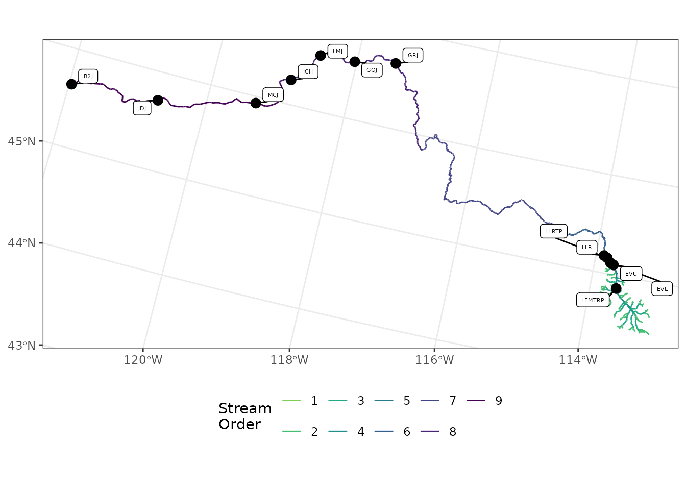
PITcleanr can make use of some of the covariates
associated with each reach in the NHDPlus_v2 layer to determine which
sites are downstream or upstream of one another. This is how we
construct the parent-child table, using the
buildParentChild() function.
# construct parent-child table
parent_child <-
  sites_sf %>%
  buildParentChild(flowlines,
                   rm_na_parent = T,
                   add_rkm = F) %>%
  editParentChild(fix_list = list(c("LMJ", "GRJ", "GOJ"))) %>%
  select(parent,
         child)
#> These child locations: B2J,
#>  had no parent location and were removed from the table.
By default, PITcleanr assumes the parent is downstream
of the child. We can switch this direction with some clever coding and
renaming.
# flip direction of parent/child relationships
parent_child <-
  parent_child %>%
  select(p = parent,
         c = child) %>%
  mutate(parent = c,
         child = p) %>%
  select(parent,
         child)
plotNodes(parent_child)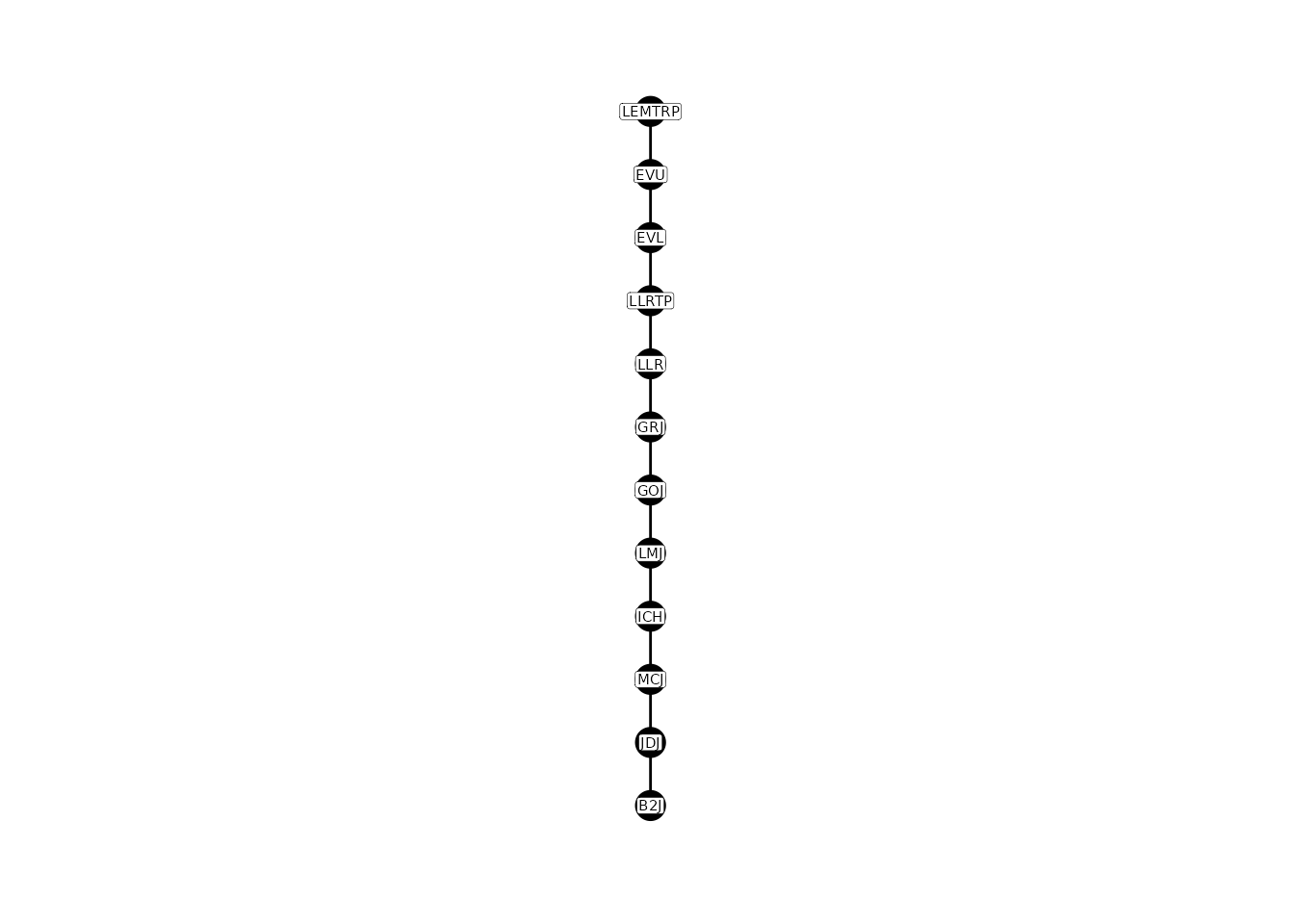
Filter Strange Capture Histories
Once the detections have been compressed, and we can describe the relationship between nodes / sites with a parent-child table, we can assign direction of a tag between two nodes. For straightforward CJS models, one of the assumptions is that fish (or whatever creature is being studied) strictly moves forward through the detection points. When a CJS model describes survival through time, that is an easy assumption to make (i.e. animals are always only moving forward in time), but when performing a space-for-time type CJS as we are discussing here, that assumption could be violated.
One way to deal with non-straightforward movements is to filter the
detections to only include those that appear to move in a
straightforward manner. PITcleanr can help the user
identify which tags have non-straightforward movements, and suggest what
detections to keep, and which ones to filter out. PITcleanr
contains a function, filterDetections(), to help determine
which tags/individuals fail to meet the one-way travel assumption and
need to be examined further. filterDetections() first runs
addDirection(), and then adds two columns, “auto_keep_obs”
and “user_keep_obs”. These are meant to indicate whether each row should
be kept (i.e. marked TRUE) or deleted (i.e. marked
FALSE). For tags that do meet the one-way travel
assumption, both “auto_keep_obs” and “user_keep_obs” columns will be
filled. If a fish moves back and forth along the same path,
PITcleanr will indicate that only the last detection at
each node should be kept.
In this analysis, we are also only concerned with tag movements after the fish has passed the Upper Lemhi rotary screw trap (site code LEMTRP). As mentioned above, some fish may have been tagged further upstream, prior to reaching LEMTRP, but we are not interested in their journey prior to LEMTRP, so we would like to filter observations of each tag prior to their detection at LEMTRP.
PITcleanr can perform multiple steps under a single
wrapper function, prepWrapper(). prepWrapper
can:
- start with a compressed detection file (
compress_obs), OR - start with the raw complete tag history (
cth_file) and then compress them. - filter out detections prior to a user-defined minimum date
(
min_obs_date) OR - filter out detections prior to a user-defined starting node
(
start_node) - add direction of movement to each detection (requires
parent_child) - note which tags have detections that follow one-way movements, and
which tags do not
- and suggest which detections to keep and which to filter out if needed,
- including detections that occur after a user-defined maximum date
(
max_obs_date)
- add a column showing all the nodes where a tag was detected if that
would be helpful to the user (
add_tag_detects; uses theextractTagObs()function fromPITcleanr) - save the output as an .xlsx or .csv file for the user to peruse with
Excel or a similar program (
save_file = TRUEandfile_namecan be set).
For our purposes, we will use the compressed detections and the parent-child table we built previously, filter for detections prior to LEMTRP and add all of the tag detections.
prepped_df <- prepWrapper(compress_obs = comp_obs,
                          parent_child = parent_child,
                          start_node = "LEMTRP",
                          add_tag_detects = T,
                          save_file = F)
In our example, we are content deleting the observations that
PITcleanr has flagged with
auto_keep_obs = FALSE.
Form Capture Histories
Often, the inputs to a CJS model include a capture history matrix,
with one row per tag, and columns of 0s and 1s describing if each tag
was detected at each time period or node. We can easily construct such
capture history matrices with the buildCapHist() function,
using all the detections we determined to keep.
# translate PIT tag observations into capture histories, one per tag
cap_hist <-
  buildCapHist(prepped_df,
               parent_child = parent_child,
               configuration = configuration)

# show an example
cap_hist
#> # A tibble: 3,622 × 2
#>    tag_code       cap_hist
#>    <chr>          <chr>
#>  1 384.1B79730415 100000000000
#>  2 384.1B7973117F 100000000000
#>  3 3D9.1C2DEF3A60 111010000000
#>  4 3DD.003D57F3DD 101001000000
#>  5 3DD.003D57F3DE 100000000000
#>  6 3DD.003D57F3DF 100000000000
#>  7 3DD.003D57F3E0 110000000000
#>  8 3DD.003D57F3E1 110000000000
#>  9 3DD.003D57F3E2 101011000000
#> 10 3DD.003D57F3E3 101000000000
#> # ℹ 3,612 more rows
To determine which position in the cap_hist string
corresponds to which node, the user can run the
defineCapHistCols() function (which is called internally
within buildCapHist()).
# to find out the node associated with each column
col_nodes <-
  defineCapHistCols(parent_child = parent_child,
                    configuration = configuration)
col_nodes
#>  [1] "LEMTRP" "EVU"    "EVL"    "LLRTP"  "LLR"    "GRJ"    "GOJ"    "LMJ"
#>  [9] "ICH"    "MCJ"    "JDJ"    "B2J"
Users have the option to keep each detection node as a separate
column when creating the capture histories, by setting
drop_nodes = F.
cap_hist2 <-
  buildCapHist(prepped_df,
               parent_child = parent_child,
               configuration = configuration,
               drop_nodes = F)
cap_hist2
#> # A tibble: 3,622 × 14
#>    tag_code      cap_hist LEMTRP   EVU   EVL LLRTP   LLR   GRJ   GOJ   LMJ   ICH
#>    <chr>         <chr>     <dbl> <dbl> <dbl> <dbl> <dbl> <dbl> <dbl> <dbl> <dbl>
#>  1 384.1B797304… 1000000…      1     0     0     0     0     0     0     0     0
#>  2 384.1B797311… 1000000…      1     0     0     0     0     0     0     0     0
#>  3 3D9.1C2DEF3A… 1110100…      1     1     1     0     1     0     0     0     0
#>  4 3DD.003D57F3… 1010010…      1     0     1     0     0     1     0     0     0
#>  5 3DD.003D57F3… 1000000…      1     0     0     0     0     0     0     0     0
#>  6 3DD.003D57F3… 1000000…      1     0     0     0     0     0     0     0     0
#>  7 3DD.003D57F3… 1100000…      1     1     0     0     0     0     0     0     0
#>  8 3DD.003D57F3… 1100000…      1     1     0     0     0     0     0     0     0
#>  9 3DD.003D57F3… 1010110…      1     0     1     0     1     1     0     0     0
#> 10 3DD.003D57F3… 1010000…      1     0     1     0     0     0     0     0     0
#> # ℹ 3,612 more rows
#> # ℹ 3 more variables: MCJ <dbl>, JDJ <dbl>, B2J <dbl>
If the user wanted to find out how many tags were detected at each node, something like the following could be run:
cap_hist2 %>%
  select(-c(tag_code,
            cap_hist)) %>%
  colSums()
#> LEMTRP    EVU    EVL  LLRTP    LLR    GRJ    GOJ    LMJ    ICH    MCJ    JDJ
#>   3622   1335   1948    257   1273    716     89     65      7     20     24
#>    B2J
#>     87
or directly from the prepared detection data:
prepped_df %>%
  group_by(node) %>%
  summarize(n_tags = n_distinct(tag_code),
            .groups = "drop") %>%
  mutate(across(node,
                ~ factor(.,
                         levels = col_nodes))) %>%
  arrange(node)
#> # A tibble: 12 × 2
#>    node   n_tags
#>    <fct>   <int>
#>  1 LEMTRP   3622
#>  2 EVU      1335
#>  3 EVL      1948
#>  4 LLRTP     257
#>  5 LLR      1273
#>  6 GRJ       716
#>  7 GOJ        89
#>  8 LMJ        65
#>  9 ICH         7
#> 10 MCJ        20
#> 11 JDJ        24
#> 12 B2J        87
Fit a Cormack-Jolly-Seber Model
Now that we’ve wrangled all our detections into capture histories,
we’re finally ready to fit a Cormack-Jolly-Seber (CJS) model. There are
many options for doing this, but in this example, we’ll use the R
package marked. Note that fitting a model like this (or
nearly any kind of model) is outside the scope of the
PITcleanr package. PITcleanr will help the
user wrangle their data into a format that can be utilized in further
analyses.
Please note that this example (which is being developed into a vignette) does not cover any of the details or assumptions behind a CJS model. Before attempting any analysis, the user should be aware of what’s involved and how to interpret the results.
The marked package requires the capture histories to be
processed and design data created. Setting the formula for
Phi (survival parameters) and p (detection
parameters) to be ~ time ensures that a separate survival
and detection parameter will be estimated between and for each site. For
further information about using the marked package, please
see the package’s CRAN
site, the package vignette,
or the paper describing it (Laake,
Johnson and Conn (2013)).
# load needed package
library(marked)

# process capture history into necessary format
cjs_proc <-
  cap_hist %>%
  select(tag_code,
         ch = cap_hist) %>%
  as.data.frame() %>%
  process.data(model = "CJS")

# create design data
cjs_ddl <-
  make.design.data(cjs_proc)

# set model construction
Phi.time <- list(formula = ~ time)
p.time <- list(formula = ~ time)

# fit model
mod1 <- crm(data = cjs_proc,
            ddl = cjs_ddl,
            model.parameters = list(Phi = Phi.time,
                                    p = p.time),
            hessian = T)
Survival and detection parameter estimates can be extracted, and the user can label them by the reaches and sites they refer to.
# pull out parameter estimates
est_preds <- predict(mod1) %>%
  map(.f = as_tibble)

est_preds$Phi <-
  est_preds$Phi %>%
  left_join(parent_child %>%
              left_join(buildNodeOrder(parent_child),
                        by = join_by(child == node)) %>%
              arrange(node_order) %>%
              mutate(occ = node_order - 1) %>%
              select(occ, parent, child) %>%
              unite(col = "reach",
                    parent,
                    child,
                    sep = "_"),
            by = join_by(occ)) %>%
  relocate(reach,
           .after = occ)

est_preds$p <-
  est_preds$p %>%
  mutate(site = rev(parent_child$child)) %>%
  relocate(site,
           .after = occ)
Now, we can plot estimate survival (Phi) and examine the
estimates in a table.
est_preds$Phi %>%
  ggplot(aes(x = fct_reorder(reach, est_preds$Phi$occ), y = estimate)) +
  geom_point() +
  geom_errorbar(aes(ymin = lcl, ymax = ucl)) +
  labs(x = "Location",
       y = "Survival")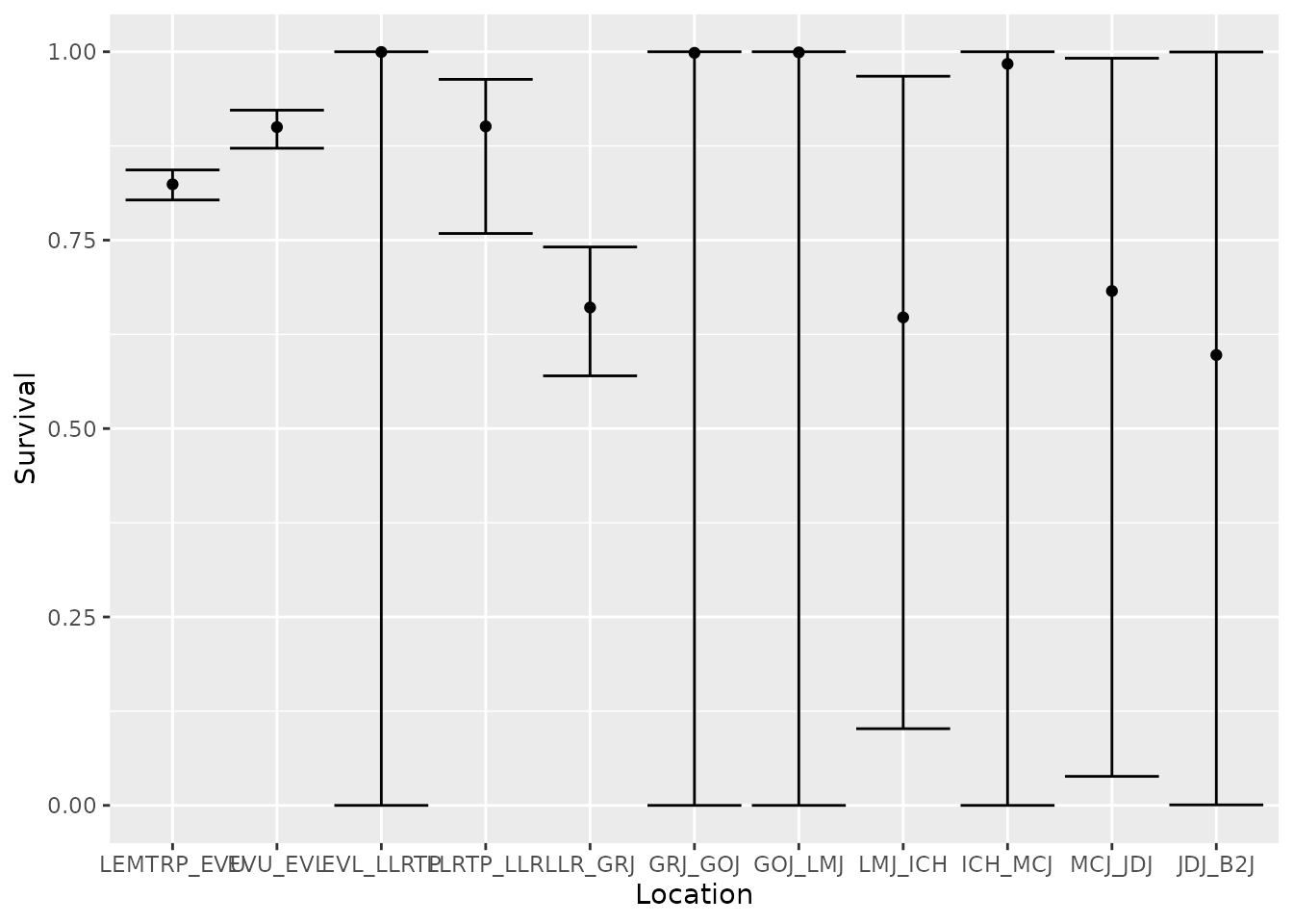
# examine the estimates
# Survival
est_preds$Phi %>%
  mutate(across(where(is.numeric),
         ~ round(., digits = 3))) %>%
  kable() %>%
  kable_styling(full_width = TRUE,
bootstrap_options = "striped")| time | occ | reach | estimate | se | lcl | ucl |
|---|---|---|---|---|---|---|
| 1 | 1 | LEMTRP_EVU | 0.824 | 0.010 | 0.803 | 0.843 |
| 2 | 2 | EVU_EVL | 0.900 | 0.013 | 0.872 | 0.922 |
| 3 | 3 | EVL_LLRTP | 1.000 | 0.047 | 0.000 | 1.000 |
| 4 | 4 | LLRTP_LLR | 0.901 | 0.048 | 0.759 | 0.963 |
| 5 | 5 | LLR_GRJ | 0.661 | 0.044 | 0.570 | 0.741 |
| 6 | 6 | GRJ_GOJ | 0.999 | 0.029 | 0.000 | 1.000 |
| 7 | 7 | GOJ_LMJ | 0.999 | 0.021 | 0.000 | 1.000 |
| 8 | 8 | LMJ_ICH | 0.648 | 0.324 | 0.102 | 0.968 |
| 9 | 9 | ICH_MCJ | 0.984 | 0.191 | 0.000 | 1.000 |
| 10 | 10 | MCJ_JDJ | 0.683 | 0.440 | 0.039 | 0.991 |
| 11 | 11 | JDJ_B2J | 0.598 | 0.945 | 0.001 | 1.000 |
We can also look at the estimates of detection probabilities.
est_preds$p %>%
  ggplot(aes(x = fct_reorder(site, est_preds$p$occ), y = estimate)) +
  geom_point() +
  geom_errorbar(aes(ymin = lcl, ymax = ucl)) +
  labs(x = "Location",
       y = "Detection")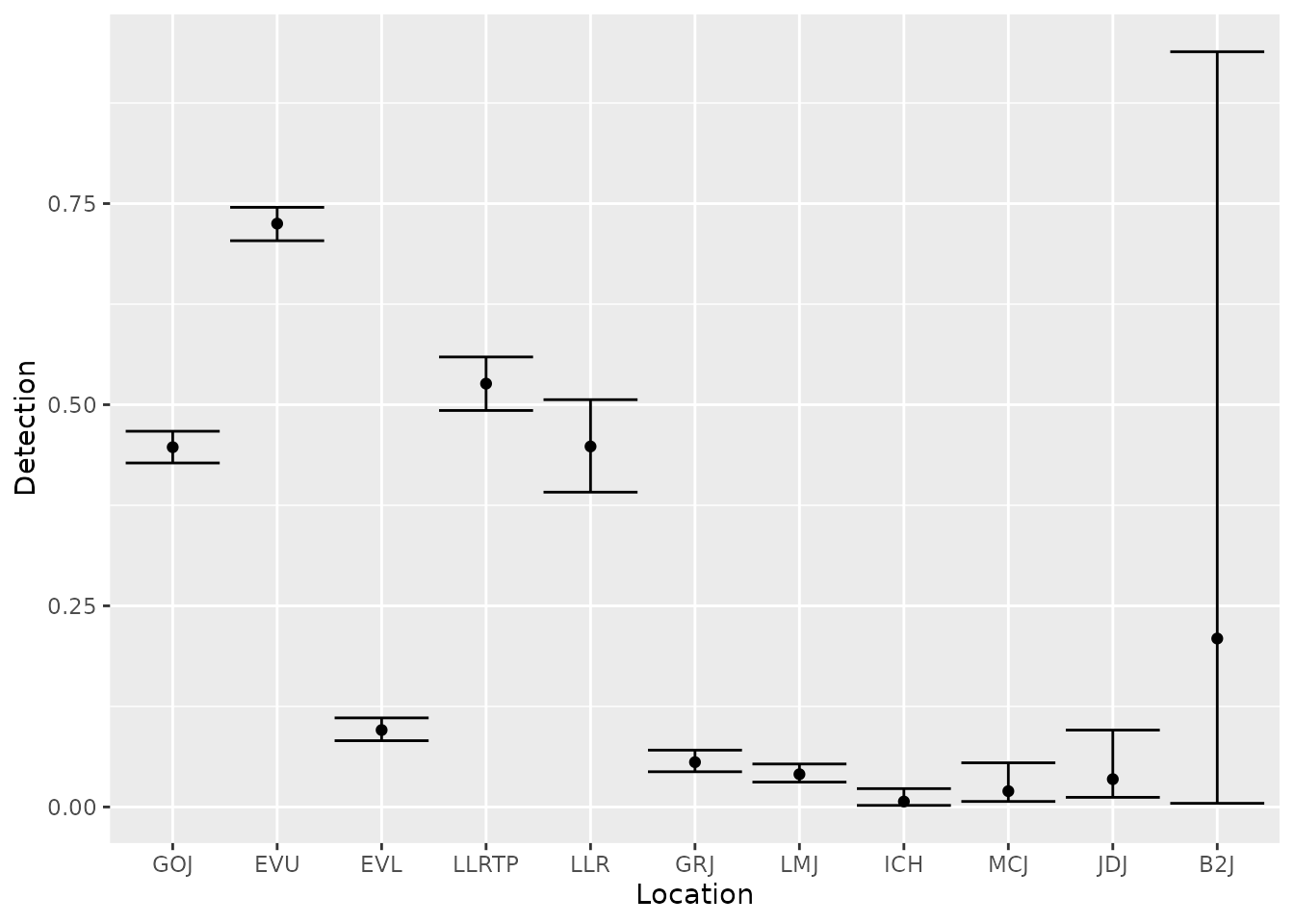
# Detection
est_preds$p %>%
  mutate(across(where(is.numeric),
         ~ round(., digits = 3))) %>%
  kable() %>%
  kable_styling(full_width = TRUE,
bootstrap_options = "striped")| time | occ | site | estimate | se | lcl | ucl |
|---|---|---|---|---|---|---|
| 2 | 2 | GOJ | 0.447 | 0.010 | 0.428 | 0.467 |
| 3 | 3 | EVU | 0.725 | 0.011 | 0.704 | 0.745 |
| 4 | 4 | EVL | 0.096 | 0.007 | 0.082 | 0.111 |
| 5 | 5 | LLRTP | 0.526 | 0.017 | 0.493 | 0.559 |
| 6 | 6 | LLR | 0.448 | 0.029 | 0.391 | 0.506 |
| 7 | 7 | GRJ | 0.056 | 0.007 | 0.044 | 0.071 |
| 8 | 8 | LMJ | 0.041 | 0.006 | 0.031 | 0.053 |
| 9 | 9 | ICH | 0.007 | 0.004 | 0.002 | 0.023 |
| 10 | 10 | MCJ | 0.020 | 0.010 | 0.007 | 0.055 |
| 11 | 11 | JDJ | 0.035 | 0.018 | 0.012 | 0.096 |
| 12 | 12 | B2J | 0.209 | 0.343 | 0.005 | 0.939 |
In this example, a user might be interested in the cumulative survival of fish from the Upper Lemhi screw trap to certain dams like Lower Granite, McNary, and John Day. These can be obtained by multiplying survival estimates up to the location of interest. Because the final survival and detection probabilities are confounded in this type of CJS model, we can’t estimate cummulative survival to Bonneville dam (B2J) unless we added detection sites either within the estuary or of adults returning to Bonneville.
# cumulative survival to Lower Granite, McNary and John Day dams
est_preds$Phi %>%
  # group_by(life_stage) %>%
  summarize(lower_granite = prod(estimate[occ <= 6]),
            mcnary = prod(estimate[occ <= 10]),
            john_day = prod(estimate[occ <= 11]))
#> # A tibble: 1 × 3
#>   lower_granite mcnary john_day
#>           <dbl>  <dbl>    <dbl>
#> 1         0.441  0.191    0.114
Warnings
Estimating fish survival is complex and requires multiple
assumptions. Be careful following this script and reproducing results
with your own data. We do not guarantee the steps listed above will
yield perfect results, and they will require adjustments to fit your
needs. The steps were only provided to get you started with
PITcleanr. Please reach out to the authors if you have
questions or need assistance using the package.