Description
When dealing with detections of individual tags, the user often is
interested in which locations are connected to which other locations
along the stream network. One way to capture this information is through
the construction of a parent-child table describing the “relationships”
among locations. In a parent-child table, each row consists of a parent
location, and a child location that is connected directly to that parent
location. By default, PITcleanr assigns parent-child
relationships as moving in an upstream direction, so a single parent may
have multiple child locations upstream, if the stream network branches
upstream of it. However, each child should only have a single parent, as
we are assuming a lack of looped connections in our stream network. If
the user is interested in a downstream parent-child relationship, the
parent and child designations in the table can
be manually switched. As an example, assuming only upstream movement, a
weir may be considered a parent and each of its next upstream arrays
considered children. A location with no detection sites further upstream
has no children, but is presumably the child of a downstream location.
All of the parent-child relationships among locations in a watershed can
describe the potential movements by an individual tag (moving from
parent to child, to the next child, etc.).
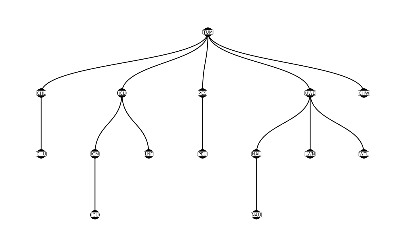
For example, in the Wenatchee River example, the parent-child table looks like this.
parent_child
#> # A tibble: 14 × 2
#>    parent child
#>    <chr>  <chr>
#>  1 TUM    CHL
#>  2 CHL    CHU
#>  3 TUM    CHW
#>  4 TUM    ICL
#>  5 ICL    ICM
#>  6 ICM    ICU
#>  7 ICL    LNF
#>  8 TUM    PES
#>  9 PES    PEU
#> 10 TUM    UWE
#> 11 UWE    LWN
#> 12 UWE    NAL
#> 13 NAL    NAU
#> 14 UWE    WTL
PITcleanr can plot these relationships graphically,
showing the relationships between parent and child sites and which ones
are connected along a single “path”. This is done using the
plotNodes() function.

Constructing a Parent-Child Table
By Hand
A user can construct a parent-child table by hand, using a .csv file
with column names parent and child. Each line
in the figure above is represented by one row in the parent-child table
listing the parent site and child site. If the user is interested in
upstream movement, the parent will be the downstream site, and every
child will have a single parent (although a parent may have multiple
children sites). If the interest is in downstream movement, then the
parent will be the upstream site.
Through Functions
When dealing with large number of sites, and many possible
connections, it can be useful to take advantage of some of
PITcleanr’s functions to construct a parent-child table.
These functions include:
-
extractSites(): based on the complete tag history (either file path and name, or the result ofreadCTH()), pulls out which sites had detections. If sites are not in PTAGIS, a configuration file should be supplied with latitude and longitudes. -
queryFlowlines(): using ansfpoint object of sites, queries the NHDPlusv2 stream layers that connect those sites. -
buildParentChild(): Based on the output fromextractSites()andqueryFlowlines(), this function constructs the parent-child table using information in the NHDPlusv2 layer about which hydrosequences are downstream of one another.
PITcleanr constructs the parent-child relationship by
joining a spatial (sf) point object of sites with the
flowlines queried via queryFlowlines(). The NHDPlus layer
that is returned contains a unique identifier, or hydrosequence, for
every segment, as well as the identifier of the hydrosequence
immediately upstream and downstream. Using this information,
PITcleanr can identify the next downstream site from every
known location (using the findDwnstrmSite() function), and
thus construct the parent child table through the
buildParentChild() function. By default,
buildParentChild() returns a tibble identifying every
parent-child pair, as well as the hydrosequence joined to the parent and
child location. If the argument add_rkm is set to
TRUE, PITcleanr will query the PTAGIS metadata
again, and attach the river kilometer (or rkm) for each parent and child
location. If the sites are not in PTAGIS, the user can join any
attributes they wish using their own configuration file.
Extracting Sites
cth_file = system.file("extdata",
                       "TUM_chnk_cth_2018.csv",
                       package = "PITcleanr",
                       mustWork = TRUE)

cth_df <- readCTH(cth_file)
The queryPtagisMeta() and buildConfig()
functions in PITcleanr return information from
all INT and MRR sites in PTAGIS. However, the user may
only be interested in detections from site codes found within their
complete tag history output, e.g., your cth_file. The
extractSites() function does just that: extracts the site
codes found in the complete tag history. In addition, the detections can
be filtered by a minimum and/or maximum detection date, and the results
are returned as either a tibble, or as a simple (spatial) feature
sf object. Setting the min_date argument could
be useful if the user is not interested in detections at sites prior to
your study period e.g., detections that occur prior to fish arriving at
your tagging or release location.
In this example, we create a new object sites_sf, return
it as an sf object (by setting as_sf = T) and
only return sites from those detections that occurred after May 1, 2018.
We also extract sites only from the Wenatchee subbasin and remove a
couple sites that we perhaps don’t care about. More information on
simple features (sf objects) can be found here.
sites_sf = extractSites(cth_file,
                        as_sf = T,
                        min_date = "20180501")

# focus on sites within Wenatchee subbasin, and drop a few sites we don't care about
sites_sf <- sites_sf %>%
  # all sites in the Wenatchee have a river kilometer that starts with 754
  filter(str_detect(rkm, "^754."),
         type != "MRR",
         site_code != "LWE") |>
  mutate(across(site_code,
                ~ recode(.,
                         "TUF" = "TUM")))
The user could create their own sf object of detection
sites, either by hand in R, or by using GIS software to create a
shapefile or geopackage that can then be read into R using the
st_read() function in the sf package. If the
user chooses this path, the file must contain at least a column called
site_code, whose values should be the same site codes found
in the configuration file. Other columns are optional. The
extractSites() function returns an sf object
with the following columns (gleaned from the configuration file):
site_codesite_namesite_typetyperkmsite_description
extractSites() will also accept a configuration file as
an argument, if the user wants to pass one of their own in. Such a file
should contain all the columns listed above.
Querying Flowlines
The user may also be interested in getting the flowlines (i.e., the
stream or river network), for their sites of interest.
PITcleanr provide the function
queryFlowlines() to accomplish that.
queryFlowlines() downloads an NHDPlus
v2 stream layer from USGS using the suggested
nhdplusTools R package. It requires the spatial location of
sites as an sf object (such as the output of
extractSites()), and a site code identified as the “root”
site. The root site might correspond with your tagging or release
location and is provided to the root_site_code argument.
The function starts from the root_site_code and downloads
all flowlines upstream from there, with a minimum stream order set by
min_strm_order.
If there are sites downstream of the root_site_code site
in the users site list, downstream flowlines will also be downloaded. By
default, the upstream and downstream flowlines will be combined into a
single sf object. However, if the user would like to keep
them separated, they can set the argument combine_up_down
to FALSE, and the downstream flowlines will be returned as
a separate element.
The queryFlowlines() function returns a list consisting
of:
-
flowlines: the flowlines upstream of theroot_site_code(and possibly the downstream ones as well) -
basin: the polygon containing the upstream flowlines
The default option (combine_up_down = TRUE) like to
combine the flowlines upstream and downstream of the root site. If the
user sets combine_up_down = FALSE, the function will return
a third element in the list called:
-
dwn_flowlines: the flowlines downstream of theroot_site_code.
Depending on the spatial extent of your flowlines, the
queryFlowlines() function may take awhile. More information
on the nhdplusTools R package can be found here.
# query the flowlines
nhd_list = queryFlowlines(sites_sf = sites_sf,
                          root_site_code = "TUM",
                          min_strm_order = 2)

# join the upstream and downstream flowlines
flowlines = nhd_list$flowlines
Mapping Sites
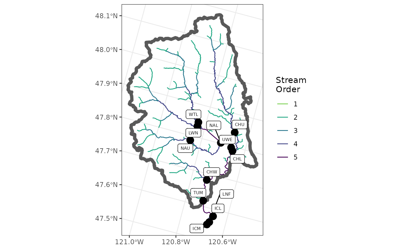
To visualize the sites and stream, the user can make a plot, such as the one in the figure below.
library(ggplot2)

ggplot() +
  geom_sf(data = flowlines,
          aes(color = as.factor(streamorde),
              size = streamorde)) +
  scale_color_viridis_d(direction = -1,
                        option = "D",
                        name = "Stream\nOrder",
                        end = 0.8) +
  scale_size_continuous(range = c(0.2, 1.2),
                        guide = 'none') +
  geom_sf(data = nhd_list$basin,
          fill = NA,
          lwd = 2) +
  geom_sf(data = sites_sf,
          size = 4,
          color = "black") +
  ggrepel::geom_label_repel(
    data = sites_sf,
    aes(label = site_code,
        geometry = geometry),
    size = 2,
    stat = "sf_coordinates",
    min.segment.length = 0,
    max.overlaps = 50
  ) +
  theme_bw() +
  theme(axis.title = element_blank())
Build Parent-Child Table
Once the user has an sf object with the spatial
locations of their sites, and a NHDPlusv2 layer of flowlines, they can
use the buildParentChild() function to construct a
parent-child table.
parent_child = buildParentChild(sites_sf,
                                flowlines)
parent_child
#> # A tibble: 12 × 4
#>    parent child parent_hydro child_hydro
#>    <chr>  <chr>        <dbl>       <dbl>
#>  1 TUM    UWE       50013200    50018330
#>  2 TUM    CHL       50013200    50022268
#>  3 TUM    CHW       50013200    50045832
#>  4 UWE    LWN       50018330    50021266
#>  5 UWE    WTL       50018330    50026363
#>  6 UWE    NAL       50018330    50028949
#>  7 CHL    CHU       50022268    50023868
#>  8 NAL    NAU       50028949    50034395
#>  9 NA     TUM             NA    50013200
#> 10 NA     LNF             NA    50016572
#> 11 NA     ICL             NA    50016572
#> 12 NA     ICM             NA    50017117
Editing Parent-Child Table
After initially building a parent-child table, there is usually some editing that needs to happen. This is necessary for a variety of reasons we’ve observed:
- Perhaps the latitude and longitude of a site was not correct, and it was placed on the wrong hydrosequence of the flowlines.
- The flowlines layer from the USGS could be inaccurate around a particular area, causing the parent-child relationships to be incorrect.
- A site may be located at the mouth of a tributary was joined to the mainstem hydrosequence of the flowline, instead of the tributary, causing problems for sites upstream and downstream of that site.
For these reasons (or any others), PITcleanr provides a
function to edit the parent-child table, editParentChild().
It requires a list the length of rows to be fixed
(fix_list). Each element of this list is a vector of length
3, where the first two elements contain the parent and child locations
to be edited, and the third element is the new (correct) parent
location. As each child contains a single parent in the table, this is
enough information to uniquely target individual rows of the
parent-child table.
The user can also switch parent-child pairs, making the parent the
child and vice versa, using the switch_parent_child
argument. This is primarily intended to fix relationships between a root
site and the initial downstream sites. If, by default, the parent child
table is built assuming upstream movement, but the user would like to
incorporate downstream movement from the root site to a location
downstream, this argument will be useful. However, it will not “fix”
associated parent-child relationships with the locations in the
switch_parent_child list; those must be fixed through the
fix_list argument.
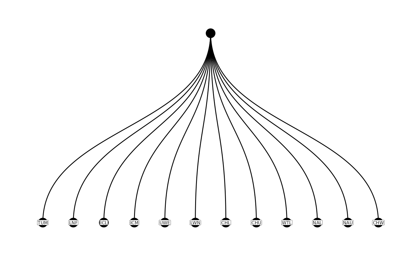
Often, a good place to start will be to examine the current
parent-child relationships using the function plotNodes().
This can help visually identify pathways that need editing.
plotNodes(parent_child)
From the figure above, the original parent-child table has some
problems with 2 sites (ICL and PES) downstream of the root site, TUM. In
addition, the flowlines are not accurate near the LNF site, or the
spatial location of that site is incorrect. We would like to make TUM
the parent of both ICL and PES, and ICL should be the parent of LNF. All
of these corrections are implemented below using the
editParentChild() function.
parent_child = editParentChild(parent_child,
                               fix_list = list(c(NA, "PES", "TUM"),
                                               c(NA, "LNF", "ICL"),
                                               c("PES", "ICL", "TUM")),
                               switch_parent_child = list(c("ICL", 'TUM')))

# view corrected parent_child table
parent_child
#> # A tibble: 12 × 4
#>    parent child parent_hydro child_hydro
#>    <chr>  <chr>        <dbl>       <dbl>
#>  1 TUM    UWE       50013200    50018330
#>  2 TUM    CHL       50013200    50022268
#>  3 TUM    CHW       50013200    50045832
#>  4 ICL    LNF       50016572    50016572
#>  5 UWE    LWN       50018330    50021266
#>  6 UWE    WTL       50018330    50026363
#>  7 UWE    NAL       50018330    50028949
#>  8 CHL    CHU       50022268    50023868
#>  9 NAL    NAU       50028949    50034395
#> 10 NA     TUM             NA    50013200
#> 11 NA     ICL             NA    50016572
#> 12 NA     ICM             NA    50017117
Incorporating Nodes
If the configuration file contains multiple nodes for some sites
(e.g., a node for each array at a site), then the parent-child table can
be expanded to accommodate these nodes using the
addParentChildNodes() function. The function essentially
“expands” (adds rows) to the existing parent-child table to accommodate
those additional nodes. Note: the addParentChildNodes()
function assumes that the parent-child table is arranged so that
children are upstream of parents, and nodes designated as
_U are upstream of those designated _D.
Currently, the function can only handle up to two nodes at each
site.
Here, we use the addParentChildNodes() function on our
existing parent_child table, and provide our existing
configuration tibble to the configuration
argument to expand the tibble. Our results are saved to a new object
parent_child_nodes.
# read in configuration file
my_configuration <- system.file("extdata",
                                "TUM_configuration.csv",
                                package = "PITcleanr",
                                mustWork = TRUE) |>
  read_csv(show_col_types = F)

# expand the parent-child table to include nodes
parent_child_nodes = addParentChildNodes(parent_child,
                                         configuration = my_configuration)

# view expanded parent-child table
parent_child_nodes
#> # A tibble: 21 × 4
#>    parent child parent_hydro child_hydro
#>    <chr>  <chr>        <dbl>       <dbl>
#>  1 TUM    UWE       50013200    50018330
#>  2 TUM    CHL_D     50013200    50022268
#>  3 TUM    CHW_D     50013200    50045832
#>  4 ICL_D  ICL_U     50016572    50016572
#>  5 ICL_U  LNF       50016572    50016572
#>  6 ICM_D  ICM_U     50017117    50017117
#>  7 UWE    LWN_D     50018330    50021266
#>  8 UWE    WTL_D     50018330    50026363
#>  9 UWE    NAL_D     50018330    50028949
#> 10 LWN_D  LWN_U     50021266    50021266
#> # ℹ 11 more rows