Introduction
This manual describes how to run the Dam Adult Branch Occupancy Model (DABOM) for adult salmon returning to a watershed. The framework typically consists of PIT tagging a representative sample of the returning adults, and using the subsequent detections of those tags at various sites upstream (or possibly downstream) of the starting location to estimate escapement or abundance past each detection site. The DABOM model estimates transition (or movement) probabilities past various detection sites while accounting for imperfect detection at those sites, essentially a multi-state variation of a spatial Cormack-Jolly-Seber model. The DABOM package implements this kind of model in a Bayesian framework. Further mathematical details of the model can be found in Waterhouse et al. (2020) which can be found here.
For this vignette, we will show a DABOM example for spring Chinook
crossing over Tumwater Dam and in the upper Wenatchee River. We start by
directing users how to query PTAGIS to get all detections of
adults at relevant observation sites (e.g., weirs, PIT tag arrays, etc.)
for a particular spawning run from a list of “valid” PIT tags.
Observation data are then “cleaned up” using the PITcleanr
R package and a final destination or spawning location is determined for
each individual. PITcleanr can also be used to prepare
detection data for use in the DABOM R package and model.
Next, we describe how to write a JAGS model for use in
DABOM, and finally, run DABOM to estimate
detection and movement probabilities within the stream network. Movement
probabilities can then be multiplied by an estimate of adult escapement
at Tumwater Dam to estimate escapement, with uncertainty, at any
observation site (or tributary) within the Wenatchee River.
We estimate escapement (or abundance) for both hatchery and natural origin fish by using both types together to estimate detection probabilities, but allow movement probabilities to vary by origin, because hatchery fish are likely moving to different areas at different rates compared to natural origin fish.
Companion R packages
DABOM has two companion R packages, PITcleanr and STADEM.
PITcleanr can assist the user in “cleaning” sometimes
unwieldy amounts of detection data from PTAGIS and preparing that detection data
for DABOM. STADEM can be used to estimate
adult escapement at a dam that, when combined with movement
probabilities from DABOM, provide an estimate of abundance
or escapement at locations of interest.
Set-up
The first step is to ensure that all appropriate software and R
packages are installed on your computer. (R) is a language and environment
for statistical computing and graphics and is the workhorse for running
all of the code and models described here. R packages are collections of
functions and data sets developed by the R community for particular
tasks. Some R packages used here are available from the general R
community (Available
CRAN Packages) whereas others (e.g., PITcleanr,
DABOM, STADEM) have been developed by the
package author and available on GitHub here.
The DABOM compendium can be downloaded as a zip from
from this URL: https://github.com/BiomarkABS/DABOM/archive/master.zip
Or the user can install the compendium as an R package from GitHub by
using Hadley Wickham’s devtools package:
# install and load remotes, if necessary
install.packages("devtools")
devtools::install_github("KevinSee/DABOM",
                         build_vignettes = TRUE)
devtools may require the downloading and installation of
Rtools. The latest version of Rtools can be found here.
For the latest development version:
devtools::install_github("KevinSee/DABOM@develop")JAGS Software
The user will also need the JAGS software to run DABOM.
They can download that from SourceForge.
JAGS (Just Another
Gibbs Sampler) software is used by
DABOM for Bayesian inference. Please download version >=
4.0.0.
Other R Packages
The user will also need to install tidyverse, a series
of R packages that work together for data science (i.e. data cleaning
and manipulation), as well as the rjags package to
interface with JAGS. The tidyverse and rjags
packages are all available from the R community and can be installed by
typing the following into your R console:
install.packages("tidyverse")
install.packages("rjags")
DABOM relies on PIT tag data that has been prepared in a
somewhat specific format. The R package PITcleanr can help
the user move from raw PIT tag detections to the type of output that
DABOM requires. Instructions for installing and using
PITcleanr can be found on the package website.
Hint: We have experienced errors installing the
PITcleanr and DABOM packages related to
“Error: (converted from warning) package ‘packagenamehere’ was built
under R version x.x.x”. Setting the following environment variable
typically suppresses the error and allows you to successfully install
the packages.
Sys.setenv(R_REMOTES_NO_ERRORS_FROM_WARNINGS = TRUE)When attempting to install PITcleanr or
DABOM you may receive an error message similar to
“there is no package called ‘ggraph’”. In that case, try to
install the given package using the following and then attempt to
install PITclean or DABOM, again.
install.packages("ggraph") # to install package from R cran
# replace ggraph with the appropriate package name as needed
PITcleanr output
Briefly, the steps to process the data for a given run or spawn year, before being ready to run DABOM, include:
- Generate valid PIT tag list
- Query PTAGIS for detections
- Develop the “river network” describing the relationship among detection sites
- Use PITcleanr to “clean up” detection data
- Review PITcleanr output to determine final capture histories
Once those steps are complete, the following lead to escapement estimates:
- Run DABOM to estimate detection and movement probabilities
- Summarize DABOM results
- Combine DABOM movement probabilities with an estimate of adult escapement at the starting node
More details about the initial preparation steps can be found in the
vignettes contained in the PITcleanr package. That vignette
can also be accessed using:
vignette("DABOM_prep",
         package = "PITcleanr")
For DABOM, the user will need
- a configuration file
- a parent-child table
- a filtered detection history (based on a PTAGIS query)
The PITcleanr package provides an example dataset we can
use to demonstrate these results. The example datasets (PTAGIS query,
configuration file and parent-child table) are installed on your
computer when you install PITcleanr. We can determine where
they are, and read them into R using the following code:
library(PITcleanr)
library(dplyr)
library(readr)
library(stringr)
library(tibble)
library(tidyr)
library(purrr)

ptagis_file = system.file("extdata",
                          "TUM_chnk_cth_2018.csv",
                          package = "PITcleanr",
                          mustWork = TRUE)

config_file = system.file("extdata",
                          "TUM_configuration.csv",
                          package = "PITcleanr",
                          mustWork = TRUE)

parent_child_file = system.file("extdata",
                                "TUM_parent_child.csv",
                                package = "PITcleanr",
                                mustWork = TRUE)


# read in parent-child table
parent_child = read_csv(parent_child_file)

# read in configuration file
configuration = read_csv(config_file)
We will now describe these components in more detail.
Configuration File
The configuration file contains all the information from PTAGIS to
map a particular detection record to a “node”. This mapping must include
the site code, the antenna code and the antenna configuration, all of
which appear in the PTAGIS query defined above. PITcleanr
provides a function to query all the metadata associated with PTAGIS
sites, and maps each array (i.e. row of antennas) at a site onto a node.
The upstream arrays are labeled with the site code plus A0
and the downstream arrays are assigned B0. For sites with
three arrays, the middle array is grouped with the upstream array. For
sites with four arrays, the upper two arrays are mapped to
A0 and the lower two arrays are mapped to B0.
However, the user can start with the ptagis_meta file and
construct this mapping any way they choose.
The key columns in a configuration file include the PTAGIS site code,
the configuration ID (related to how the various antennas are laid out
at a site), the antenna ID and the DABOM node that antenna is assigned
to. The first three are included with PTAGIS queries of capture
histories, and the inclusion of the node column allows
PITcleanr to map every detection to a node.
Parent-Child Table
The parent-child table describes the stream network in terms of which detection locations are connected to each other. A parent-child table defines the closest previous detection location (parent) for each detection location (child). If a tag is seen at a child location, it must have moved past the parent location. For adult salmonid movement, the parent location is downstream of the child location. Each child location may only have a single parent, but a parent location may have multiple child locations due to the branching nature of the stream network.
To run DABOM, a parent-child table must include the following columns:
-
parent: generally the PTAGIS site code of the parent location -
child: generally the PTAGIS site code of the child location -
parent_hydro: the hydrosequence of the NHDPlus layer where the parent location is -
child_hydro: the hydrosequence of the NHDPlus layer where the child location is -
parent_rkm: the river kilometer of the parent location (generally queried from PTAGIS) -
child_rkm: the river kilometer of the child location (generally queried from PTAGIS)
Graphically, these relationships are shown in the figure below.
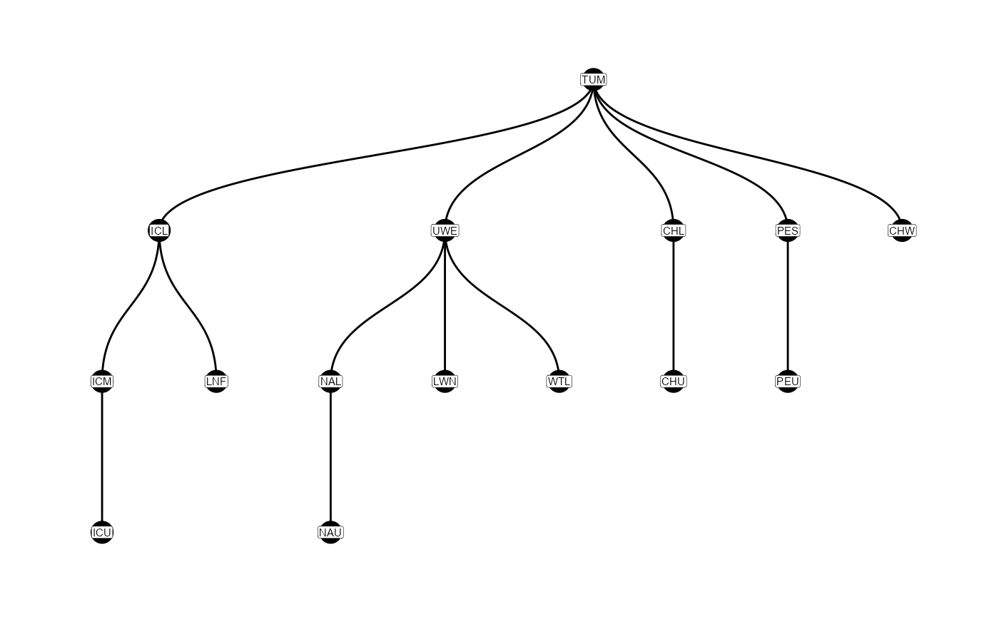
Graphical representation of the parent-child table, showing which sites are upstream of others. Tags start at TUM, and move down the figure.
Filtered Capture History
One of the assumptions in the DABOM model is that fish are making a one-way upstream migration, which ends in their spawning location. At every branching site (with multiple possible upstream paths), the fish can only move up one of those paths in the model. So if a fish is detected moving past one site and later seen moving past a different site that implies the fish swam back downstream then turned up a different tributary, both of those observations cannot be kept in the model. Before running DABOM, a user will need to “clean” the detection histories of the tags and decide if there are multiple detections like those described above which one to keep.
PITcleanr can take the raw detections from PTAGIS,
assign each to a node (based on the configuration file), compress them,
add directionality (based on the parent-child table), and flag those
tags with detections in multiple branches. For each detection,
PITcleanr adds two columns to indicate whether each
detection should be retained for DABOM: auto_keep_obs and
user_keep_obs. For tags with straightforward detections
(i.e. all detections appear to have one-way directional movement), the
added columns auto_keep_obs and user_keep_obs
will be marked TRUE. For tags with less straightforward
movement patterns, PITcleanr assumes that the last
detection with movement noted as “forward” or “unknown” (or “start”) is
the spawning location, and attempts to mark the
auto_keep_obs column as TRUE for the last
detections along that movement path. For these tags,
prepWrapper returns NA’s in the
user_keep_obs column.
We’ve identified the output from PTAGIS provided by
PITcleanr (ptagis_file). Now we can compress
those observations and prepare them for DABOM. Note that in the
prepWrapper function, we have added the detection nodes
(not just site codes) to the parent-child table, using the
addParentChildNodes function from PITcleanr.
The prepWrapper function also includes a minimum and
maximum observed date (min_obs_date and
max_obs_date, in YYYYMMDD format) so the user
can filter out observations before a certain date (e.g. detections of
fish marked as juveniles, detections at mainstem dams prior to reaching
the release point, etc.) and after a certain date (e.g. detections of
kelts swimming downstream after spawning, carcasses drifting downstream
after spawning, ghost detections in subsequent years, etc.).
prepped_ch = PITcleanr::prepWrapper(cth_file = ptagis_file,
                                    file_type = "PTAGIS",
                                    configuration = configuration,
                                    parent_child = parent_child %>%
                                      addParentChildNodes(configuration = configuration),
                                    min_obs_date = "20180301",
                                    max_obs_date = "20180930")
The first 10 rows of the prepped_ch file look like:
| tag_code | node | slot | event_type_name | n_dets | min_det | max_det | duration | travel_time | start_date | node_order | path | direction | auto_keep_obs | user_keep_obs |
|---|---|---|---|---|---|---|---|---|---|---|---|---|---|---|
| 384.3B239AC47B | TUM | 1 | Recapture | 1 | 2018-06-16 15:26:31 | 2018-06-16 15:26:31 | 0 mins | 184.0167 mins | 2018-06-16 15:26:31 | 1 | TUM | start | TRUE | TRUE |
| 384.3B239AC47B | UWE | 2 | Observation | 1 | 2018-06-23 22:03:13 | 2018-06-23 22:03:13 | 0 mins | 10476.7000 mins | 2018-06-16 15:26:31 | 2 | TUM UWE | forward | TRUE | TRUE |
| 384.3B239AC47B | NAL_U | 3 | Observation | 1 | 2018-07-01 00:06:16 | 2018-07-01 00:06:16 | 0 mins | 10203.0500 mins | 2018-06-16 15:26:31 | 4 | TUM UWE NAL_D NAL_U | forward | TRUE | TRUE |
| 3DD.003B9DD720 | TUM | 1 | Recapture | 1 | 2018-06-17 09:39:26 | 2018-06-17 09:39:26 | 0 mins | 216.6500 mins | 2018-06-17 09:39:26 | 1 | TUM | start | TRUE | TRUE |
| 3DD.003B9DD725 | TUM | 1 | Recapture | 1 | 2018-06-19 09:33:08 | 2018-06-19 09:33:08 | 0 mins | 722.4167 mins | 2018-06-19 09:33:08 | 1 | TUM | start | TRUE | TRUE |
| 3DD.003B9DD725 | CHU_U | 2 | Observation | 1 | 2018-06-28 21:34:58 | 2018-06-28 21:34:58 | 0 mins | 13681.8333 mins | 2018-06-19 09:33:08 | 5 | TUM CHL_D CHL_U CHU_D CHU_U | forward | TRUE | TRUE |
| 3DD.003B9DDAB0 | TUM | 1 | Recapture | 1 | 2018-07-17 11:51:44 | 2018-07-17 11:51:44 | 0 mins | 183.4500 mins | 2018-07-17 11:51:44 | 1 | TUM | start | TRUE | TRUE |
| 3DD.003B9F123C | TUM | 1 | Recapture | 1 | 2018-06-21 09:45:14 | 2018-06-21 09:45:14 | 0 mins | 288.0167 mins | 2018-06-21 09:45:14 | 1 | TUM | start | TRUE | TRUE |
| 3DD.003B9F123C | UWE | 2 | Observation | 1 | 2018-07-01 12:55:31 | 2018-07-01 12:55:31 | 0 mins | 14590.2833 mins | 2018-06-21 09:45:14 | 2 | TUM UWE | forward | TRUE | TRUE |
| 3DD.003BC7A654 | TUM | 1 | Recapture | 1 | 2018-06-09 22:36:03 | 2018-06-09 22:36:03 | 0 mins | 420.6000 mins | 2018-06-09 22:36:03 | 1 | TUM | start | TRUE | TRUE |
The next step would be for a user to filter the prepared data for all
rows with user_keep_obs == NA, and then fill in the
user_keep_obs column by hand for each detection node. These
decisions could be guided by the auto_keep_obs column
(PITcleanr’s best guess), but could also be informed by the
date of detections and the user’s biological knowledge of the system.
Before sending the data along to DABOM, all the missing
user_keep_obs rows should be filled out as either
TRUE or FALSE. The user can then remove all
the rows where user_keep_obs == FALSE. For our example,
we’ll accept all the auto_keep_obs recommendations.
This step may be easier to perform outside of R. The
prepWrapper function has the ability to save the output to
a .csv or .xlsx file which the user can then open with other software,
such as Excel. Once the user has replaced all the NAs or
blanks in the user_keep_obs column with TRUE
or FALSE, they can read that file back into R. The code to
do this looks like this:
prepped_ch = PITcleanr::prepWrapper(cth_file = ptagis_file,
                                    file_type = "PTAGIS",
                                    configuration = configuration,
                                    parent_child = parent_child %>%
                                      addParentChildNodes(configuration = configuration),
                                    min_obs_date = "20180301",
                                    max_obs_date = "20180930",
                                    save_file = T,
                                    file_name = "C:/Users/USERNAME/Desktop/PITcleanr_output.xlsx")

# after the user has ensured all the user_keep_obs rows are TRUE or FALSE
filter_ch = readxl::read_excel("C:/Users/USERNAME/Desktop/PITcleanr_output.xlsx") %>%
  filter(user_keep_obs)
Finally, we’ll need to know the origin (hatchery or wild/naturally
produced) of each tag. This involves constructing a tibble with two
columns: tag_code and origin. The user might
be able to do this based on data taken when tagging the fish, or it
could be constructed from the PTAGIS file:
fish_origin = suppressMessages(read_csv(ptagis_file)) %>%
  select(tag_code = `Tag Code`,
         origin = `Mark Rear Type Name`) %>%
  distinct() %>%
  mutate(origin = str_sub(origin, 1, 1),
         origin = recode(origin,
                         "U" = "W"))

fish_origin
#> # A tibble: 1,406 × 2
#>    tag_code       origin
#>    <chr>          <chr>
#>  1 384.3B239AC47B W
#>  2 3DD.003B9DD720 H
#>  3 3DD.003B9DD725 W
#>  4 3DD.003B9DDAB0 W
#>  5 3DD.003B9F123C H
#>  6 3DD.003BC7A654 H
#>  7 3DD.003BC7F0E3 H
#>  8 3DD.003BC80A3C H
#>  9 3DD.003BC80D81 H
#> 10 3DD.003BC80F20 H
#> # ℹ 1,396 more rows
DABOM currently has the ability to handle up to two
types of fish (e.g. hatchery and wild). Therefore, the
origin column of fish_origin should only
contain a maximum of two distinct entries. Note that in the example
above, we have marked all the fish with “Unknown” or “U” origin as wild,
to conform to this. It is fine if all the fish have the same origin
(e.g. all are wild).
Now our data is ready for DABOM.
Write JAGS Model
The DABOM model is implemented in a Bayesian framework, using JAGS
software. JAGS requires a model file (.txt format) with specific types
of syntax. See the JAGS user manual for more detail about JAGS models.
The DABOM package contains a function to write this model
file, based on the relationships defined in the parent-child table, and
how nodes are mapped to sites in the configuration file.
library(DABOM)

# file path to the default and initial model
basic_mod_file = tempfile("DABOM_init", fileext = ".txt")

writeDABOM(file_name = basic_mod_file,
           parent_child = parent_child,
           configuration = configuration)
If the user would like the initial transition parameters (chances of
moving along one of the initial branches from the starting point) to be
time-varying, meaning they will shift as the season goes on,
writeDABOM has an argument, time_varying which
can be set to TRUE. This can be important when the group of
tagged fish may not be representative of the total run, perhaps because
the trap rate shifted over the course of the run and there exists
differential run timing between fish going to those initial branches.
For example, this situation often occurs at Lower Granite dam, so the
initial movement parameters are allowed to shift on a weekly basis. This
reduces the bias in the estimates, but will take longer to run, and does
require estimates of total escapement for each strata (e.g. week) of the
movement parameters.
Modify JAGS Model
Often the user will have a parent-child table based on all the
detection sites they are interested in using. However, there may have
been no fish detected at some of those sites that year. Rather than let
the model churn away on estimating parameters that have no data to
inform them, we have devised a function to “turn off” some parameters.
Some of these parameters are specific to the origin of the fish, such as
turning off movement parameters past a particular site only for hatchery
fish, if no hatchery fish were observed there, so the
fish_origin input is required.
This includes setting the detection probability to 0 for nodes that
had no detections (or were not in place during the fishes’ migration),
setting the detection probability to 100% for nodes that function as
single arrays with no upstream detection sites (because there is no way
to estimate detection probability there), and fixing some movement
probabilities to 0 if no tags were observed along that branch. Setting
the detection probability to 100% may lead to a conservative estimate of
escapement past that particular site (i.e. escapement was at
least this much), but since many terminal sites are further
upstream in the watershed, where most detection probabilities are likely
close to 100% already, this may not be a bad assumption to make. The
function fixNoFishNodes updates the initial JAGS file with
these improvements, writes a new JAGS .txt file, and sends a message to
the user about what it has done.
# filepath for specific JAGS model code for species and year
final_mod_file = tempfile("DABOM_final", fileext = ".txt")

# writes species and year specific jags code
fixNoFishNodes(init_file = basic_mod_file,
               file_name = final_mod_file,
               filter_ch = filter_ch,
               parent_child = parent_child,
               configuration = configuration,
               fish_origin = fish_origin)
#> Fixed the following sites at 0% detection probability, because no tags were observed there:
#>   CHL_D, ICU_D, ICU_U, PES_D, PES_U, PEU_D, PEU_U .
#>
#> Fixed the following nodes at 100% detection probability, because it is functioning as a single array with no upstream detections:
#>   LNF .
#>
#>
#> Fixed movement upstream of the following sites to 0 because no detections upstream:
#>   ICM, PES .
Run JAGS Model
To run the JAGS model, we need to set some initial values, create inputs in a format conducive to JAGS, and set which parameters we would like to track.
Set Initial Values
The only initial values we need to set are for where tags are in the system, based on their observed detections. Otherwise, JAGS could randomly assign them an initial value of being in one tributary, when they are actually observed in another, which will cause JAGS to throw an error and crash.
# Creates a function to spit out initial values for MCMC chains
init_fnc = setInitialValues(filter_ch = filter_ch,
                            parent_child = parent_child,
                            configuration = configuration)
Create JAGS Input
JAGS requires the data to be input in the form of a list. The
writeDABOM function has also assumed a particular format
and names for the data inputs. So DABOM has a function to
transform the data into the right format expected by JAGS:
# Create all the input data for the JAGS model
jags_data = createJAGSinputs(filter_ch = filter_ch,
                             parent_child = parent_child,
                             configuration = configuration,
                             fish_origin = fish_origin)
If the user is running a time-varying version of DABOM, they will
need to add some additional data as input, namely the number of temporal
strata (i.e. weeks) and which strata each tag falls into (i.e. which
week did they cross the initial dam?). This can be done after running
createJAGSinputs, by using the addTimeVaryData
function:
# add data for time-varying movement
jags_data = c(jags_data,
              addTimeVaryData(filter_ch = filter_ch,
                              start_date = "20180301",
                              end_date = "20180630"))
Set Parameters to Save
The user needs to tell JAGS which parameters to track and save
posterior samples for. Otherwise, the MCMC algorithms will run, but the
output will be blank. Based on the model file, DABOM will
pull out all the detection and movement parameters to track:
# Tell JAGS which parameters in the model that it should save.
jags_params = setSavedParams(model_file = final_mod_file)
If the user is running a time-varying version of DABOM, the function
setSavedParams does have an input,
time_varying, which can be set to TRUE. This
will add the variance parameter related to the random walk of those
time-varying movement parameters, in case the user is interested in
tracking that.
Run MCMC
R users have developed several different packages that can be used to
connect to the JAGS software and run the MCMC algorithm. Here, we will
present example code that uses the rjags package, which was
written by the author of the JAGS software. First, the user runs an
adaptation or burn-in phase, which requires the path to the JAGS model
file, the input data, any initial values function, the number of MCMC
chains to run and the number of adaptation iterations to run. To test
that the model is working, a user may set n.chains = 1 and
n.adapt to a small number like 5, but to actually run the
model we recommend:
n.chains = 4n.adapt = 5000
To make the results fully reproducible, we recommend setting the
random number generator seed in R, using the set.seed()
function. This will ensure the same MCMC results on a particular
computer, although the results may still differ on different
machines.
library(rjags)
set.seed(5)

jags = jags.model(file = final_mod_file,
                  data = jags_data,
                  inits = init_fnc,
                  n.chains = 4,
                  n.adapt = 5000)
If this code returns a message
Warning message: Adaptation incomplete, this indicates
further burn-in iterations should be run, which the user can do by
“updating” the jags object using this code (and setting the
n.iter parameter to something large enough):
update(jags,
       n.iter = 1000)
Finally, once the adaptation or burn-in phase is complete, the user
can take MCMC samples of the posteriors by using the
coda.samples function. This is where the user tells JAGS
which parameters to track. The user can also set a thinning paramater,
thin, which will save every nth sample, instead of all of
them. This is useful to avoid autocorrelations in the MCMC output.
Again, we would recommend the following settings:
n.iter = 5000thin = 10
Across four chains, this results in (5000 samples / 10 (every 10th sample) * 4 chains) 2000 samples of the posteriors.
dabom_samp_tum = coda.samples(model = jags,
                              variable.names = jags_params,
                              n.iter = 5000,
                              thin = 10)
Results
We have included an example of posterior samples with the
DABOM package, to save the user time when testing the
package. It can be accessed by running:
data("dabom_samp_tum")Detection Probability Estimates
If a user is interested in the estimates of detection probability,
estimated at every node in the DABOM model, the DABOM
package provides a simple function to extract these,
summariseDetectProbs(). The output includes the number of
distinct tags observed at each node, as well as the mean, median, mode
and standard deviation of the posterior distribution. It also includes
the highest posterior density interval (HPDI) of whatever \(\alpha\)-level the user desires (using the
cred_int_prob argument), the default value of which is 95%.
The HPDI is the narrowest interval of the posterior distribution that
contains the \(\alpha\)-level mass, and
is the Bayesian equivalent of a confidence interval.
# summarize detection probability estimates
detect_summ = summariseDetectProbs(dabom_mod = dabom_samp_tum,
                                   filter_ch = filter_ch,
.cred_int_prob = 0.95)| node | n_tags | mean | median | mode | sd | skew | kurtosis | lower_ci | upper_ci |
|---|---|---|---|---|---|---|---|---|---|
| CHL_U | 472 | 0.474 | 0.474 | 0.470 | 0.017 | 0.008 | 2.796 | 0.440 | 0.504 |
| CHU_D | 316 | 0.637 | 0.638 | 0.643 | 0.029 | -0.059 | 2.810 | 0.579 | 0.693 |
| CHU_U | 269 | 0.543 | 0.543 | 0.535 | 0.028 | -0.118 | 2.948 | 0.489 | 0.599 |
| CHW_D | 19 | 0.952 | 0.965 | 0.987 | 0.044 | -1.674 | 6.976 | 0.866 | 1.000 |
| CHW_U | 19 | 0.951 | 0.965 | 0.986 | 0.046 | -1.713 | 7.086 | 0.861 | 1.000 |
| ICL_D | 1 | 0.097 | 0.083 | 0.062 | 0.065 | 1.167 | 4.587 | 0.003 | 0.230 |
| ICL_U | 1 | 0.099 | 0.088 | 0.050 | 0.063 | 1.108 | 4.733 | 0.002 | 0.220 |
| ICM_D | 10 | 0.839 | 0.859 | 0.912 | 0.101 | -0.933 | 3.878 | 0.650 | 0.995 |
| ICM_U | 11 | 0.918 | 0.938 | 0.980 | 0.076 | -1.580 | 6.371 | 0.770 | 1.000 |
| LNF | 6 | 1.000 | 1.000 | 1.000 | 0.000 | NaN | NaN | 1.000 | 1.000 |
| LWN_D | 13 | 0.623 | 0.632 | 0.657 | 0.126 | -0.245 | 2.781 | 0.391 | 0.872 |
| LWN_U | 12 | 0.577 | 0.584 | 0.592 | 0.126 | -0.148 | 2.690 | 0.354 | 0.832 |
| NAL_D | 116 | 0.450 | 0.450 | 0.451 | 0.034 | -0.019 | 3.054 | 0.385 | 0.515 |
| NAL_U | 116 | 0.450 | 0.450 | 0.443 | 0.035 | 0.024 | 2.873 | 0.385 | 0.517 |
| NAU_D | 132 | 0.985 | 0.987 | 0.991 | 0.011 | -1.426 | 5.930 | 0.964 | 1.000 |
| NAU_U | 130 | 0.969 | 0.972 | 0.979 | 0.015 | -1.097 | 5.145 | 0.938 | 0.994 |
| TUM | 1406 | NA | NA | NA | NA | NA | NA | NA | NA |
| UWE | 272 | 0.765 | 0.765 | 0.764 | 0.022 | -0.168 | 3.155 | 0.725 | 0.811 |
| WTL_D | 16 | 0.624 | 0.627 | 0.631 | 0.097 | -0.190 | 2.806 | 0.441 | 0.811 |
| WTL_U | 23 | 0.886 | 0.901 | 0.918 | 0.073 | -1.042 | 4.063 | 0.740 | 0.993 |
| CHL_D | 0 | 0.000 | 0.000 | 0.000 | 0.000 | NaN | NaN | 0.000 | 0.000 |
| ICU_D | 0 | 0.000 | 0.000 | 0.000 | 0.000 | NaN | NaN | 0.000 | 0.000 |
| ICU_U | 0 | 0.000 | 0.000 | 0.000 | 0.000 | NaN | NaN | 0.000 | 0.000 |
| PES_D | 0 | 0.000 | 0.000 | 0.000 | 0.000 | NaN | NaN | 0.000 | 0.000 |
| PES_U | 0 | 0.000 | 0.000 | 0.000 | 0.000 | NaN | NaN | 0.000 | 0.000 |
| PEU_D | 0 | 0.000 | 0.000 | 0.000 | 0.000 | NaN | NaN | 0.000 | 0.000 |
| PEU_U | 0 | 0.000 | 0.000 | 0.000 | 0.000 | NaN | NaN | 0.000 | 0.000 |
Estimate Escapement
To estimate escapement past each detection point, DABOM requires two things: an estimate of the movement or transition probability past that point, and an estimate of the total escapement somewhere in the stream network. Most of the time, that estimate of total escapement is provided at the tagging or release site (e.g. Tumwater Dam), and we’ll assume that’s what is available for this example.
Compile Transition Probabilities
Compiling the transition probabilities is both a matter of ensuring
that the parameters from JAGS match the site codes of each detection
point (so that movement past CHL is named as such), but also multiplying
some transition probabilities together when appropriate. For instance,
the ultimate probability that a tag moves past CHU is the probability of
moving from TUM past CHL, and then from CHL past CHU. These
multiplication steps are done in the compileTransProbs()
function, which takes the MCMC output from JAGS and uses the
parent-child table and configuration file to
determine which parameters to multiply together. So it is a generic
function that could be applied to any DABOM model a user writes.
move_post <- extractTransPost(dabom_mod = dabom_samp_tum,
                              parent_child = parent_child,
                              configuration = configuration)

trans_df = compileTransProbs(trans_post = move_post,
                             parent_child = parent_child)
The resulting tibble contains a column describing the MCMC chain that
sample is from (chain) the overall iteration of that sample
(iter), the origin, either one or two
(origin), the parameter (param) which is coded
such that the site code refers to the probability of moving past that
site, and the value of the posterior sample (value). Some
parameters end in _bb, which refers to the tags that moved
past a particular branching node, but did not move into one of the
subsequent branches. The “bb” stands for “black box”, meaning we’re not
sure exactly what happened to those fish. They have spawned in an area
above that branching node, but below upstream detection points, they may
have died in that area (due to natural causes or fishing) or they may
have moved downstream undetected and were not seen at any other
detection sites.
Total Escapement
In our example, at Tumwater Dam, every fish that moves upstream of the dam is physically moved upstream, after being identified as hatchery or wild. Therefore, the total escapement, by origin, at Tumwater is known precisely, with no standard error (for 2018, there were 317 natural origin Chinook and 1,167 hatchery Chinook). The user can input that by setting up a tibble with origin and total escapement.
tot_escp = tibble(origin_nm = c("Wild", "Hatchery"),
                  origin = c(1,2),
                  tot_escp = c(317, 1167),
                  tot_escp_se = c(31.5, 122.8))
Each of the transition probabilities can then be multiplied by this
total escapement, resulting in posterior samples of escapement or
abundance past each detection site. If there is any uncertainty in the
total escapement, we recommend bootstrapping samples of the total
escapement with the appropriate mean and standard error (using the same
number of bootstrap samples as they have posterior samples of transition
probabilities), labeling those bootstraps with a chain number,
chain, and an iteration number, iter.
tot_escp_boot <-
  tot_escp |>
  crossing(chain = unique(trans_df$chain)) |>
  group_by(origin_nm,
           origin,
           chain) |>
  reframe(tot_esc_samp = map2(tot_escp,
                                tot_escp_se,
                                .f = function(x, y) {
                                  tibble(tot_abund = rnorm(max(trans_df$iter),
                                                           mean = x,
                                                           sd = y)) %>%
                                    mutate(iter = 1:n())
                                })) |>
  unnest(cols = tot_esc_samp)
These bootstrapped estimates of total escapement function like the
MCMC posterior draws of an abundance model, and can be matched with the
movement posterior draws in trans_df to calculate abundance
at each location. Use the calcAbundPost() function for this
operation.
escp_post <-
  calcAbundPost(move_post = trans_df,
                abund_post = tot_escp_boot)
These draws can then be summarized using the
summarisePost() function, or the user could summarize the
posterior samples however they wish.
escp_summ <- summarisePost(escp_post,
                           abund,
                           location = param,
                           origin_nm,
origin)| location | origin_nm | origin | mean | median | mode | sd | skew | kurtosis | lower_ci | upper_ci |
|---|---|---|---|---|---|---|---|---|---|---|
| CHL | Wild | 1 | 216.9 | 216.6 | 219.8 | 24.3 | 0.1 | 3.0 | 170.4 | 265.9 |
| CHL_bb | Wild | 1 | 77.6 | 77.0 | 75.7 | 14.6 | 0.2 | 2.9 | 50.1 | 107.1 |
| ICL | Wild | 1 | 1.8 | 1.6 | 0.8 | 1.3 | 1.6 | 7.5 | 0.1 | 4.3 |
| NAL | Wild | 1 | 52.2 | 51.7 | 50.2 | 8.8 | 0.3 | 2.9 | 35.5 | 69.5 |
| NAL_bb | Wild | 1 | 22.2 | 21.7 | 19.6 | 5.7 | 0.6 | 3.2 | 12.0 | 33.6 |
| NAU | Wild | 1 | 30.0 | 29.6 | 28.8 | 5.9 | 0.3 | 3.1 | 18.9 | 41.5 |
| CHL | Hatchery | 2 | 830.8 | 830.6 | 826.5 | 88.6 | 0.0 | 2.9 | 654.6 | 999.8 |
| CHL_bb | Hatchery | 2 | 453.2 | 452.4 | 452.5 | 52.5 | 0.1 | 3.0 | 349.4 | 554.3 |
| ICL | Hatchery | 2 | 19.8 | 19.2 | 17.9 | 5.1 | 0.5 | 3.3 | 10.9 | 30.7 |
| NAL | Hatchery | 2 | 217.0 | 215.9 | 213.7 | 27.6 | 0.2 | 3.0 | 165.1 | 270.8 |
| NAL_bb | Hatchery | 2 | 108.8 | 107.9 | 104.6 | 17.5 | 0.3 | 3.1 | 75.9 | 143.4 |
| NAU | Hatchery | 2 | 108.2 | 107.4 | 104.5 | 15.5 | 0.3 | 3.1 | 77.7 | 137.8 |
Time-Varying Versions (GRA)
For DABOM models with time-varying parameters (e.g. Lower Granite Dam), calculating escapement estimates is a little more complicated. Essentially the user needs to extract the movement probabilities along each initial branch for each strata (e.g. week), and multiply those by an estimate of total escapement at the release point for that strata. Those estimates by strata can then be summed for each branch across all strata, to estimate total escapement to each initial branch across the entire run. Those branch escapement estimates are then multiplied by the subsequent movement or transition probabilities within that branch to estimate escapement past all detection points within each branch.
Here, we start by compiling only the time-varying movement parameters.
# read in the LGR parent-child table
pc_lgr <-
  system.file("extdata",
              "LGR_parent_child.csv",
              package = "PITcleanr",
              mustWork = TRUE) |>
  read_csv(show_col_types = F)

# read in the LGR configuration file
config_lgr <-
  system.file("extdata",
              "LGR_configuration.csv",
              package = "PITcleanr",
              mustWork = TRUE) |>
  read_csv(show_col_types = F)

# load the MCMC draws from the DABOM model for LGR
data("dabom_samp_lgr")

trans_post <- extractTransPost(dabom_mod = dabom_samp_lgr,
                               parent_child = pc_lgr,
                               configuration = config_lgr) |>
  # focus only on wild fish
  filter(origin == 1)

# compile main branch movement parameters
main_post <-
  compileTransProbs(trans_post,
                    parent_child = pc_lgr,
                    time_vary_only = T,
                    time_vary_param_nm = "strata_num")
For Lower Granite, total unique wild escapement can be estimated with
the STate-space Adult
Dam Eescapement Model
(STADEM), which interacts well with DABOM to generate all these
estimates. If the user has posterior samples from a STADEM model that
was set up with the same strata as DABOM, those can be extracted by
using the extractPost() function from the
STADEM package.
library(STADEM)
data("stadem_mod")

# posteriors of STADEM abundance by strata_num
abund_post <-
  STADEM::extractPost(stadem_mod,
                      param_nms = c("X.new.wild",
                                    "X.new.hatch")) |>
  mutate(origin = case_when(str_detect(param, "wild") ~ 1,
                            str_detect(param, "hatch") ~ 2,
                            .default = NA_real_)) |>
  rename(abund_param = param) |>
  filter(origin == 1)

# escapement to each main branch across whole season
main_escp <-
  calcAbundPost(move_post = main_post,
                abund_post = abund_post,
                time_vary_param_nm = "strata_num")
The movement probabilities within non-main branches (so those without time-varying parameters) are compiled separately.
# compile tributary branch movement parameters
branch_post <-
  compileTransProbs(trans_post,
                    parent_child = pc_lgr,
                    time_vary_only = F)
These are then combined with the main-branch escapements using the
calcAbundPost() function again. The main-branch abundance
posteriors can be row-bound to the tributary abundance posteriors to
track abundance across all locations. These draws can then be summarized
using the summarisePost() function.
# estimate escapement to all tributary sites
trib_escp <-
  calcAbundPost(branch_post,
                main_escp |>
                  rename(main_branch = param,
                         tot_abund = abund),
                .move_vars = c("origin",
                               "main_branch",
                               "param"),
                .abund_vars = c("origin",
                                "main_branch"))

# combine main-branch and tributary draws into a single object
all_escp_post <-
  trib_escp |>
  select(-value) |>
  bind_rows(main_escp |>
              mutate(main_branch = param,
                     tot_abund = abund)) |>
  arrange(chain,
          iter,
          origin,
          main_branch,
          param)

all_escp_summ <-
  all_escp_post |>
  summarisePost(value = abund,
                main_branch,
                origin,
                param)
all_escp_summ |>
  filter(mean > 0,
         main_branch == "LLR") |>
  rename(location = param) |>
  mutate(across(mean:mode,
                round)) |>
  kable(digits = 1,
caption = "Summary statistics of escapement estimates to all locations within one main-branch, the Lemhi River (site LLR).")| main_branch | origin | location | mean | median | mode | sd | skew | kurtosis | lower_ci | upper_ci |
|---|---|---|---|---|---|---|---|---|---|---|
| LLR | 1 | EVL | 113 | 112 | 108 | 18.8 | 0.2 | 2.9 | 77.3 | 149.7 |
| LLR | 1 | EVL_bb | 3 | 2 | 1 | 3.3 | 2.4 | 10.6 | 0.0 | 9.6 |
| LLR | 1 | EVU | 110 | 109 | 112 | 18.4 | 0.3 | 3.0 | 77.0 | 147.9 |
| LLR | 1 | EVU_bb | 3 | 2 | 1 | 2.7 | 1.7 | 6.8 | 0.0 | 8.1 |
| LLR | 1 | HYC | 52 | 51 | 49 | 12.4 | 0.4 | 3.0 | 30.8 | 77.4 |
| LLR | 1 | LLR | 153 | 153 | 155 | 22.0 | 0.2 | 2.8 | 112.0 | 197.3 |
| LLR | 1 | LLR_bb | 41 | 40 | 38 | 10.7 | 0.5 | 3.3 | 20.8 | 61.9 |
| LLR | 1 | LRW | 55 | 54 | 54 | 12.9 | 0.5 | 3.2 | 32.3 | 81.9 |
| LLR | 1 | LRW_bb | 55 | 54 | 54 | 12.9 | 0.5 | 3.2 | 32.3 | 81.9 |
It is important to note that the user is responsible for ensuring
that the strata used in STADEM and that used in DABOM are the same. The
addTimeVaryData() function uses a function from the
STADEM package to generate strata on a weekly basis, so as
long as the inputs are the same, the strata will be identical. However,
if the user wishes to use strata from a different model (not STADEM),
that are not set up to be weekly (e.g. uneven lengths, split across
known changes in trap rates, etc.), it is fairly easy to generate the
n_strata and dam_strata inputs to JAGS without
using the addTimeVaryData() function, but then they must
also generate estimates of escapement (by origin if necessary) for each
strata. Then it is also upon the user to combine those estimates
(bootstrapped if necessary due to uncertainty) with the appropriate
transition probability posteriors.
Updating a DABOM Model
As new detection sites are installed, the current DABOM models may
need to change. The user can modify the configuration file and
parent-child table through R, or manually in other software like Excel
and then read those files back into R. Once the configuration file and
parent-child table are updated, the other functions in the
DABOM package will work correctly with these updated files,
including writeDABOM, fishNoFishNodes,
setInitialValues, createJAGSinputs and
setSavedParams. The user can run the JAGS model, and even
pull out summaries of the detection probabilities using
summariseDetectProbs, and generate transition probabilities
using extractTransPost and
compileTransProbs.